|
收稿日期: 2016-11-21; 优先数字出版日期: 2017-09-01
基金项目: 北京市科委项目(编号:238796489321);国家自然科学基金(编号:41501396)
第一作者简介: 彭波(1991— ),男,硕士研究生,研究方向为高光谱图像异常探测。E-mail:pengbo@radi.ac.cn
通讯作者简介: 张立福(1967— ),男,研究员,研究方向为高光谱遥感机理及典型应用。E-mail:zhanglf@radi.ac.cn
中图分类号: TP751
文献标识码: A
|
摘要
传统的实时异常探测算法需对高维的背景样本统计矩阵进行求逆运算,数值稳定性差、时间复杂度高。而基于Cholesky分解,将高维矩阵的求逆运算转换为求解下三角线性系统,采用Cholesky分解因子的一阶修正方法快速更新背景统计信息,降低逐像元实时处理的时间复杂度并且保持数值稳定性。由于算法仅涉及下三角矩阵的更新过程,压缩了数据存储空间,适用于机载或星上实时处理。采用3维接收器曲线(3D-ROC)以及计算机实际处理时间对实验结果进行定量化分析,结果表明,该算法在不降低异常探测精度的同时,对当前时刻像元的实时处理时间约缩短为基于QR分解算法的0.4%—0.65%,或减少至基于Woodbury矩阵引理算法的27%—33%,有效提高实时高光谱异常探测器的计算性能,并且保持处理过程中的数值稳定性。
关键词
高光谱, 异常探测, 实时处理, Cholesky分解, 一阶修正
Abstract
Anomaly detection is one of the most important issues in hyperspectral remote sensing. However, traditional anomaly detection algorithms cannot be used for onboard real-time processing due to heavy computational load caused by the dimensionality curse of hyperspectral data. To implement onboard real-time hyperspectral anomaly detection, the following must be performed: (1) conduct the process in a causal progressive manner without any future data relative to the pixel under test; (2) output the result for each sample right after collecting it; (3) process the data with constant theoretical computational complexity. The present widely used algorithms generally employ QR decomposition or Woodbury’s Identity for real-time anomaly detection. However, their computational load is still extremely high. Also, they suffered serious numerical instabilities led by runoff error in the matrix inverting process. The main objective of this study is to further accelerate the real-time detection process and avoid the matrix inversion module to maintain numerical stabilities. In this work, we proposed a novel real-time sample-wise hyperspectral anomaly detection algorithm based on Cholesky decomposition. The background sample correlation matrix and covariance matrix were symmetric positive definite, which can be factored into a lower triangular matrix and its transpose. We modified the background suppression process into a process that finds the solution to a lower-triangular linear system based on this characteristic. Furthermore, the real-time process is significantly accelerated by virtue of rank-1 updates to the Cholesky factor of the background statistical matrix. Moreover, the numerical stabilities were maintained. Finally, we performed a three dimensional ROC (3D-ROC) analysis to evaluate the performance of real-time anomaly detection in terms of background suppression, detection power, false alarm, and the relationship between each other. An experiment on an actual hyperspectral dataset collected by Field Imaging Spectrometer System (FISS) revealed the following. (1) The proposed algorithm significantly reduced the computing time to process the incoming data. The theoretical computational load demonstrated high efficiency of the technique developed in this work. The time consumption for each incoming sample was reduced to 0.4%—0.65% of the time consumed by traditional QR decomposition-based algorithms, and 27%—33% of the time corresponding to Woodbury’s identity-based techniques. (2) The sample varying background suppression provided an acceptable visual inspection of the anomalies. Real-time processing prevented these weak signals from being suppressed by later detected strong signals. Additionally, 3D-ROC analysis could effectively evaluate the detection performance of hyperspectral anomaly detectors. The real-time sample-wise hyperspectral anomaly detector developed in this study is not only computationally efficient but also numerically stable, significantly contributing to onboard implementations.
Key words
hyperspectral, anomaly detection, real-time processing, Cholesky decomposition, rank-1 updating
1 引 言
异常探测是高光谱遥感的重要应用之一(Chang,2003)。利用高光谱图像数据进行异常探测需求解压制后的背景统计信息,即样本协方差矩阵K(Reed和Yu,1990)或自相关矩阵R(Chang和Chiang,2002)的逆矩阵K–1或R–1。由于高光谱数据波段多,数据处理耗时较长,传统异常探测算法无法满足实时处理的时效性要求,如火灾火点与移动目标的实时探测。实时高光谱异常探测能够在成像光谱仪获取数据的过程中,对当前时刻所获取的待测样本立即进行快速处理,无须等待研究区所有数据获取完毕,并且实时处理的时间复杂度恒定且较短,不随数据量的增长而增长,有效提高高光谱目标探测的在线处理与应用能力。
针对摆扫型成像光谱仪(如AVIRIS)逐像元采集数据的方式,目前高光谱异常探测的实时处理方法主要为:(1) 基于背景矩阵QR分解的方法,可避免直接求解K–1或R–1,在保持数值计算精度的同时降低异常探测的计算复杂度(Chang 等,2001;Chang和Hsueh,2006;Du和Zhang,2011;Molero 等,2013)。(2) 基于卡尔曼滤波器的思想,利用Woodbury矩阵引理(Du和Nekovei,2009;Acito 等,2011;Chen 等,2014;Rossi 等,2014;Chang 等,2015),结合上一时刻K–1或R–1与当前时刻所获取的像元,递归求解当前时刻所需K–1或R–1,该方法避免采用所有像元进行重复计算,降低背景压制过程的时间消耗。需要注意的是,基于多核处理器平台(FPAG,多DSP,GPU)的并行计算方法(Paz和Plaza,2010;Guo 等,2014;Zhao 等,2014)并不是实时处理,而是快速处理。
传统的实时高光谱异常探测算法存在时间复杂度高以及数值稳定性差的问题。一方面,由于计算机舍入误差的存在,基于Woodbury矩阵引理的递归算子对K–1或R–1进行低阶修正时易造成严重的数值精度损失(Stewart,1998;http://infoscience. epft.ch/record/161458[2016-11-21]),在机载或星上成像光谱仪不断获取数据并进行实时处理的过程中,该损失会一直存在,并且在后续探测过程中不断累积,造成严重的数值计算错误,同时,该递归算子涉及多次矩阵与向量之间的乘积操作,空间、时间等消耗依然较大。另一方面,基于矩阵QR分解的实时处理算法虽然避免了矩阵求逆运算,但该方法在实时处理过程中,每一次对当前时刻K或R进行分解所需时间复杂度为O(n3) (n为高光谱数据波段数量),由于高光谱数据波段较多,该方法计算代价仍较高。
基于以上问题,提出一种新型的逐像元实时高光谱异常探测算法,论证高光谱遥感图像背景统计矩阵的正定对称性结构,利用Cholesky分解及其分解因子的一阶修正方法,将背景压制过程转换为下三角线性系统求解过程,快速更新当前时刻所需背景统计量,保证数值计算的稳定性,降低实时处理的时间与空间复杂度,且探测精度保持不变。
2 传统异常探测
经典高光谱异常探测(AD)算法RX(Reed和Yu,1990)以全局样本像元的协方差矩阵K作为背景统计量,记作K-AD。以全局样本像元的自相关矩阵R(Chang和Chiang,2002)为背景统计信息的异常探测算法考虑到样本一阶统计量的影响,记作R-AD。设
2.1 K-AD和R-AD
K-AD采用背景样本协方差矩阵,可表示为
|
${\delta ^{{\rm{K}} - {\rm{AD}}}}\left( {{{{r}}_i}} \right) = {\left( {{{{r}}_i} - {{\mu }}} \right)^{\rm{T}}}{{{K}}^{ - 1}}\left( {{{{r}}_i} - {{\mu }}} \right) \lessgtr \eta$
|
(1) |
式中,
R-AD (Chang和Chiang,2002)采用样本自相关矩阵
|
${\delta ^{{\rm{R}} - {\rm{AD}}}}\left( {{{{r}}_i}} \right) = {{r}}_i^{\rm{T}}{{{R}}^{ - 1}}{{{r}}_i} \lessgtr \eta$
|
(2) |
式中,
2.2 因果式R-AD与K-AD
由于R-AD与K-AD需要探测区域所有样本数据参与背景估计,而逐像元实时异常探测要求背景统计信息随当前时刻所采集的样本进行实时更新。需要注意的是,术语“因果”强调了在实时处理过程中,仅能采用当前时刻已获取的数据进行异常探测,未被获取的像元不能参与计算。
假设rn为成像光谱仪当前时刻所获取的第n个样本,R(n)为当前时刻已获取的n个样本的自相关矩阵,即
|
${\delta ^{{\rm{CR}} - {\rm{AD}}}}\left( {{{{r}}_n}} \right) = {{r}}_n^{\rm{T}}{{{R}}^{ - 1}}\left( n \right){{{r}}_n}$
|
(3) |
式中,
基于样本协方差矩阵的异常探测算法K-AD需要计算样本一阶统计量,即样本均值向量μ。假设μ(n)为当前时刻已获取的n个样本的均值向量,即
|
${\delta ^{{\rm{CK}} - {\rm{AD}}}}\left( {{{{r}}_n}} \right) = {\left[ {{{{r}}_n} - {{\mu }}\left( n \right)} \right]^{\rm{T}}}{{{K}}^{ - 1}}\left( n \right)\left[ {{{{r}}_n} - {{\mu }}\left( n \right)} \right]$
|
(4) |
随着所采集数据量的不断增大,对背景统计矩阵的估计与压制时间将不断增长,限制了当前时刻对新获取像元进行实时处理的速度(Zhao 等,2015)。
3 实时异常探测
通过对上一时刻背景统计矩阵的Cholesky分解因子进行一阶修正,在恒定时间复杂度内递归计算当前时刻背景统计信息,可有效提高实时高光谱异常探测效率。
3.1 CR-AD实时处理
3.1.1 线性系统输出异常
为提高实时处理速度及数值稳定性,基于背景自相关矩阵的数据结构特性,对异常探测过程进行优化。首先,式(2)中背景自相关矩阵为对称矩阵;其次,假设x为任意B×1维非零矢量,可得
|
$\begin{array}{l}{{{x}}^{\rm{T}}}{{R}}(n){{x}} = {{{x}}^{\rm{T}}}\left[ {\left( {1/n} \right)\sum\limits_{i{\rm{ = 1}}}^n {{{{r}}_i}{{r}}_i^{\rm{T}}} } \right]{{x}}\\ = \left( {1/n} \right)\sum\limits_{i{\rm{ = 1}}}^n {{{\left( {{{r}}_i^{\rm{T}}{{x}}} \right)}^{\rm{T}}}\left( {{{r}}_i^{\rm{T}}{{x}}} \right)} \\ = \left( {1/n} \right)\sum\limits_{i{\rm{ = 1}}}^n {{{\left\| {{{r}}_i^{\rm{T}}{{x}}} \right\|}^{\rm{2}}}} \geqslant 0\end{array}$
|
(5) |
式(5)表明自相关矩阵R(n)为半正定对称矩阵,其特征值
|
${e_i} > 0\;\;\left( {i = 1,2, \cdots ,B} \right)$
|
(6) |
因此,R(n)为对称正定矩阵。充分利用该特性将有效提高CR-AD的实时处理效率与数值计算精度。
进一步地,基于R(n)的正定对称性,利用Cholesky分解,可将R(n)快速分解为一个下三角矩阵与其转置矩阵的乘积
|
${{R}}\left( n \right) = {{{C}}_n}{{C}}_n^{\rm{T}}$
|
(7) |
式中,Cn为B×1维下三角矩阵。该分解过程能够最大限度保持数值稳定性(Stewart,1998;Seeger,2004),减少对后续实时异常探测精度的影响。
为避免当前时刻待测像元rn对背景估计的影响,防止rn被背景R(n)所压制,每一次获取新像元之后,采用上一时刻背景统计信息R(n–1)对rn进行探测处理(Chang,2016)。对CR-AD进行改写,可得实时CR-AD,记作RCR-AD
|
$\begin{array}{l}{\delta ^{{\rm{RCR - AD}}}}\left( {{{{r}}_n}} \right) = {{r}}_n^{\rm{T}}{{{R}}^{ - 1}}\left( {n - 1} \right){{{r}}_n}\\[7pt] = {{r}}_n^{\rm{T}}{\left[ {{{{C}}_{n - 1}}{{C}}_{n - 1}^{\rm{T}}} \right]^{ - 1}}{{{r}}_n}\\[7pt] = {\left( {{{C}}_{n - 1}^{ - 1}{{{r}}_n}} \right)^{\rm{T}}}\left( {{{C}}_{n - 1}^{ - 1}{{{r}}_n}} \right)\\[7pt] = {\left\| {{{{z}}_n}} \right\|^2}\end{array}$
|
(8) |
式中,
基于式(8),求解出zn即可输出当前时刻rn的异常响应值。值得注意的是,为保证数值稳定性以及加速求解过程,并不需要对下三角矩阵Cn进行求逆运算,改写
|
${{{C}}_{n - 1}}{{{z}}_n} = {{{r}}_n}$
|
(9) |
式(9)为下三角线性方程组系统,利用前向迭代可快速求解出zn,具体求解过程如下
|
${{{z}}_n}\left( k \right) = \frac{{{{{r}}_n}\left( k \right) - \sum\limits_{l = 1}^{k - 1} {{{{C}}_{n - 1}}\left( {k,l} \right){{{z}}_n}\left( l \right)} }}{{{{{C}}_{n - 1}}\left( {k,k} \right)}},\;k = \left( {1,2, \cdots ,B} \right)$
|
(10) |
式中,zn(k)与rn(k)分别表示向量zn与rn中第k个元素,
3.1.2 背景优化与实时更新
为实时处理下一时刻所获取样本,需在恒定且较短时间内更新当前时刻背景统计量R(n)
|
$\begin{aligned}{{R}}(n) = & \left( {1/n} \right)\sum\limits_{i = 1}^n {{{{r}}_i}{{r}}_i^{\rm{T}}} = & \left( {1 - 1/n} \right){{R}}(n - 1) + \left( {1/n} \right){{{r}}_n}{{r}}_n^{\rm{T}}\end{aligned}$
|
(11) |
式中,R(n–1)为当前时刻已知的前(n–1)个像元的样本自相关矩阵,rn为当前时刻新获取的样本。
由式(8)中RCR-AD可知,每一次对rn进行实时处理时,仅需提供上一状态下R(n–1)的Cholesky分解因子
假设
如式(11),R(n)由上一时刻R(n–1)以及当前时刻rn更新所得。由于矩阵
|
$\begin{aligned}{{R}}(n) = & \left( {1 - 1/n} \right)\left[ {{{R}}(n - 1) + \left( {1/(n - 1)} \right){{{r}}_n}{{r}}_n^{\rm{T}}} \right] =\\ & \left( {1 - 1/n} \right)[{{R}}(n - 1) + {{{\tilde{{r}}}}_n}{\tilde{{r}}}_n^{\rm{T}}] =\\ & \left( {1 - 1/n} \right)[{{{C}}_{n - 1}}{{C}}_{n - 1}^{\rm{T}} + {{{\tilde{{r}}}}_n}{\tilde{{r}}}_n^{\rm{T}}] =\\ & \left( {1 - 1/n} \right){{{\tilde{{C}}}}_n}{\tilde{{C}}}_n^{\rm{T}} = {{{C}}_n}{{C}}_n^{\rm{T}}\end{aligned}$
|
(12) |
式中,
3.2 CK-AD实时处理
根据3.1.1中证明过程,结合样本协方差矩阵的构造方式,容易得出K(n)同样为对称正定矩阵。设K(n)的Cholesky分解为
|
$\begin{aligned}{\delta ^{{\rm{RCK - AD}}}}\left( {{{r}}_n} \right) = & {\left[ {{{{r}}_n} - {{\mu}} \left( n \right)} \right]^{\rm{T}}}{{{K}}^{ - 1}}\left( {n - 1} \right)\left[ {{{{r}}_n} - {{\mu}} \left( n \right)} \right] = \\ & \tilde {{r}}_n^{\rm{T}}{\left[ {{{{L}}_{n - 1}}{{L}}_{n - 1}^{\rm{T}}} \right]^{ - 1}}{{\tilde {{r}}}_n} = \\ & {\left( {{{L}}_{n - 1}^1{{\tilde {{r}}}_n}} \right)^{\rm{T}}}\left( {{{L}}_{n - 1}^{ - 1}{{\tilde {{r}}}_n}} \right) = {\left\| {{{{z}}_n}} \right\|^2}\end{aligned}$
|
(13) |
式中,
如式(13),RCK-AD的实时处理方式比RCR-AD更复杂。当前时刻获取像元数据rn后,首先需要对样本均值μ(n)进行更新,μ(n)由上一时刻均值μ(n–1)与当前时刻rn计算所得
|
$\begin{aligned}{{\mu }}(n) = & \left( {1/n} \right)\sum\limits_{i = 1}^n {{{{r}}_i}} {\rm{ = }}\left( {1/n} \right)\sum\limits_{i = 1}^{n - 1} {{{{r}}_i}} + \left( {1/n} \right){{{r}}_n} = \\ & \left[ {1 - \left( {1/n} \right)} \right]\left[ {1/\left( {n - 1} \right)\sum\limits_{i = 1}^{n - 1} {{{{r}}_i}} } \right] + \left( {1/n} \right){{{r}}_n} = \\ & \left[ {1 - \left( {1/n} \right)} \right]{{\mu }}(n - 1) + \left( {1/n} \right){{{r}}_n}\end{aligned}$
|
(14) |
进一步,对背景协方差矩阵K(n)进行改写
|
$\begin{aligned}{{K}}\left( n \right) = & \frac{1}{n}\sum\limits_{i = 1}^n {\left[ {{{{r}}_i} - {{\mu }}\left( n \right)} \right]{{\left[ {{{{r}}_i} - {{\mu }}\left( n \right)} \right]}^{\rm{T}}}} = \\ & \frac{1}{n}\sum\limits_{i = 1}^n {{{{r}}_i}{{r}}_i^{\rm{T}} - {{\mu }}\left( n \right){{{\mu }}^{\rm{T}}}\left( n \right)} = \\ &{{R}}\left( n \right) - {{\mu }}\left( n \right){{{\mu }}^{\rm{T}}}\left( n \right)\end{aligned}$
|
(15) |
考虑到
|
$\begin{aligned}{{K}}\left( n \right) = & {{{L}}_n}{{L}}_n^{\rm{T}}{\rm{ = }}{{R}}\left( n \right) - {{\mu }}\left( n \right){{{\mu }}^{\rm{T}}}\left( n \right) =\\ & {{{C}}_n}{{C}}_n^{\rm{T}} - {{\mu }}\left( n \right){{{\mu }}^{\rm{T}}}\left( n \right)\end{aligned}$
|
(16) |
式中,
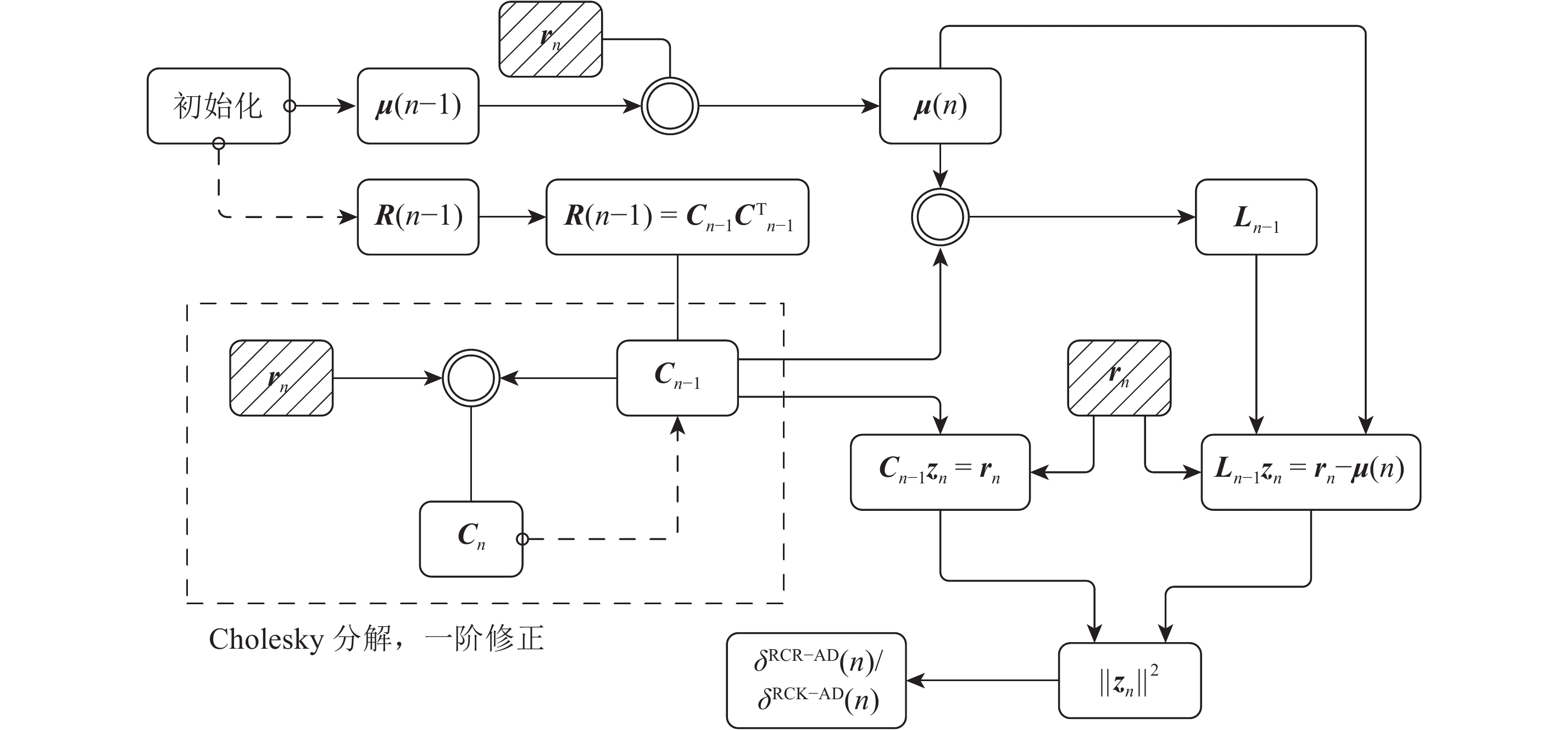
图1为RCR-AD以及RCK-AD的实时处理流程。
3.3 时间复杂度分析
实时异常探测对算法计算性能要求苛刻,对RCR-AD及RCK-AD进行时间复杂度分析有助于评价探测器的计算性能。时间复杂度以处理过程中的计算机浮点数运算次数(flops)作为衡量指标。

不考虑背景样本自相关矩阵的初始Cholesky分解过程,RCR-AD算法可分为两个部分:
(1) 获取待测像元rn后,结合已知的R(n–1)的Cholesky分解因子
(2) 为下一时刻探测所需,对
因此,RCR-AD实时处理每一个当前时刻像元所需时间复杂度总计为3.5B2 flops。
RCK-AD在RCR-AD处理过程的基础上,需首先去除一阶统计量μ(n),如式(15),该过程需要2.5B2 flops。因此,RCK-AD算法实时处理当前时刻新获取的像元数据所需时间复杂度总计为6B2 flops。
值得注意的是,若不采用Cholesky分解因子一阶修正方法,对每一次更新所得背景统计矩阵R(n)或K(n)重新进行Cholesky分解,仅该分解过程所需时间复杂度即为O(B3) flops(Press 等,2007)。因此,本算法大大降低实时异常探测的时间消耗。同时,因背景统计矩阵的重复求逆过程易引入严重的舍入误差(Stewart,1998;Seeger,2004),本算法无需进行求逆运算,保持了数据处理的数值稳定性。
4 实验结果与分析
为验证所提出算法的时效性,采用实验室采集的高光谱图像数据进行计算机仿真测试。测试环境为64位Windows 10系统,Intel CoreTM i7-6770HQ 2.59 GHz CPU,仿真实验平台为Visual Studio C++ 2015。
4.1 实验室FISS数据
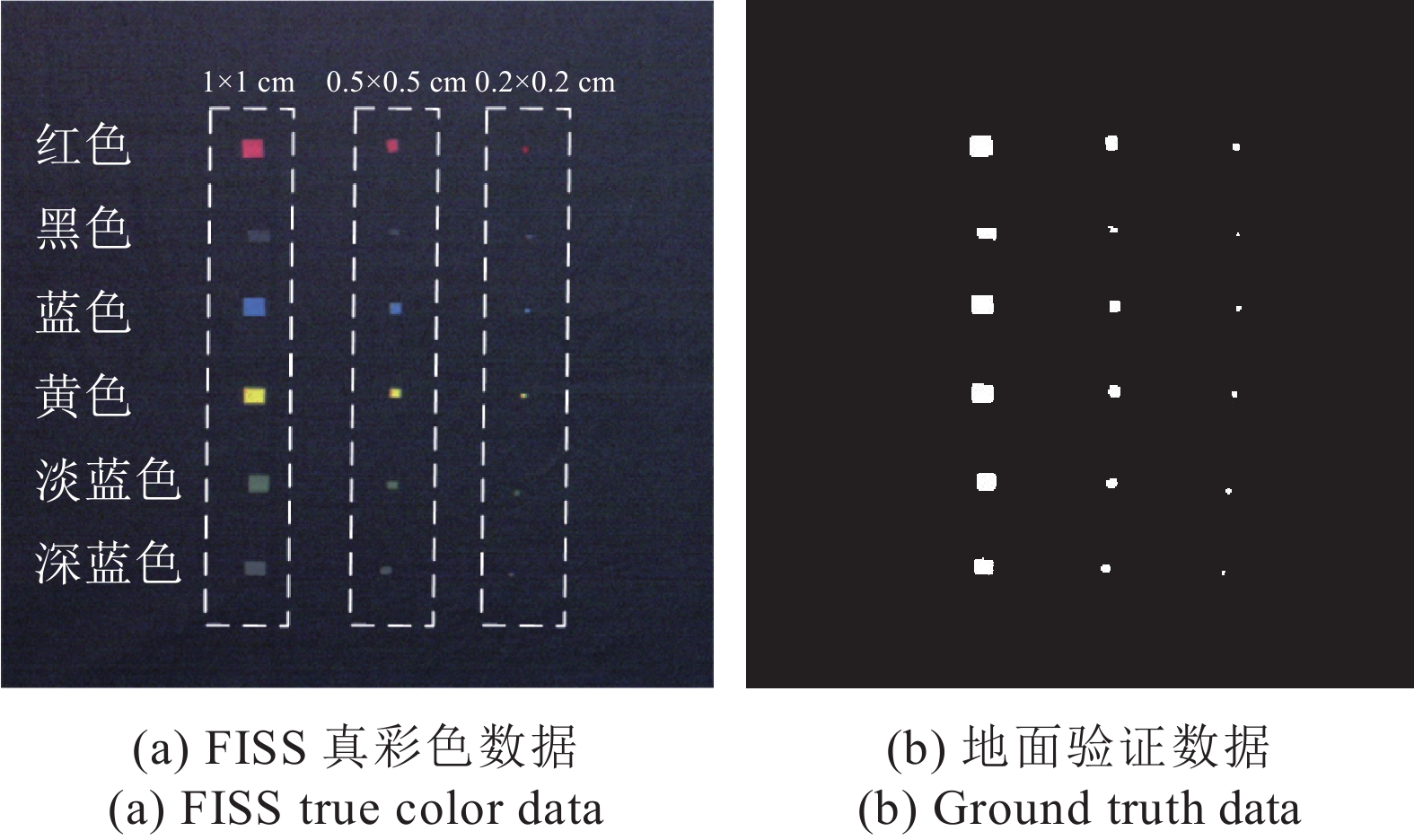
采用的FISS数据由地面成像光谱辐射测量系统FISS在实验室采集,该系统由中国科学院遥感与数字地球研究所于2008年自主研发完成。其光谱范围为379—870 nm,共344个连续波段,光谱分辨率优于5 nm,空间分辨率为1 mrad。经过数据预处理,去除信噪比较低的波段(1—34,325—334),剩余290个波段进行仿真实验。
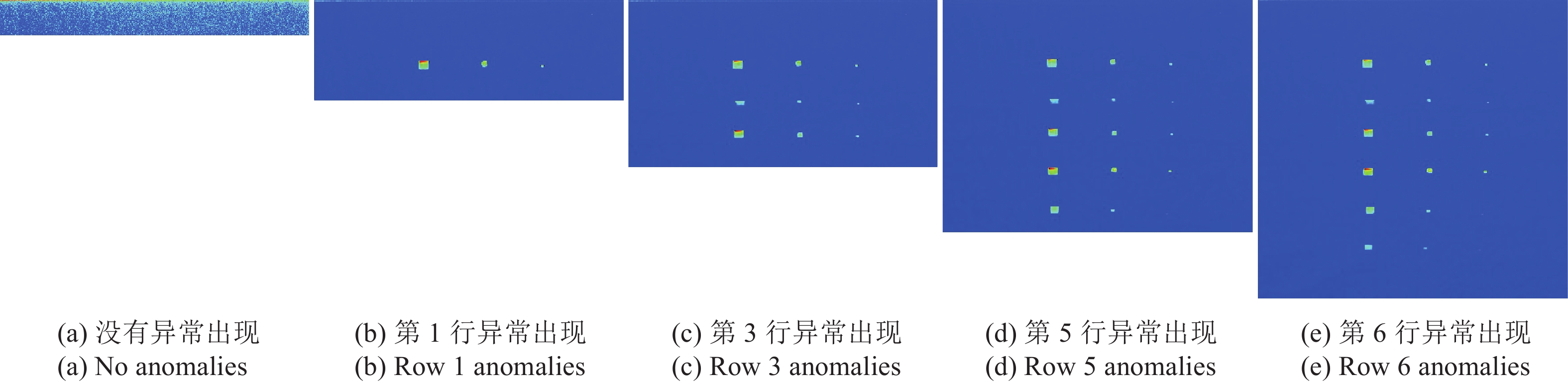
图2为FISS测试数据,其中图2(a)为该数据真彩色合成图,共18个不同尺寸(1×1 cm,0.5×0.5 cm,0.2×0.2 cm)的人工目标均匀排列在一块黑色纺织布料上。目标中第1—4行为纸质目标,分别为红色(PRed)、黑色(PBla)、蓝色(PBlu)和黄色(PYel),第5—6行为纺织布料目标,分别为淡蓝色(FLGr)和深蓝色(FDGr)。图2(b)为标记目标位置的地面验证数据。
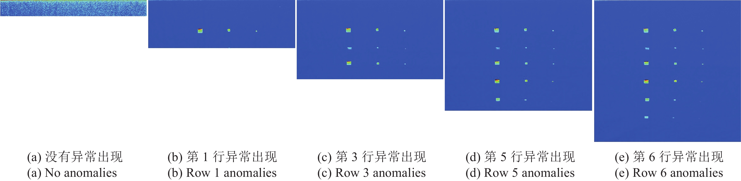
4.2 实时异常探测结果
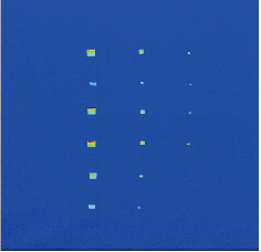
利用实时异常探测算法(RCR-AD、RCK-AD)对上述FISS数据进行仿真处理,图3和图4为实时异常探测过程示意图。为便于目视判读,探测结果经过非线性拉伸,灰度值转换到dB空间,即灰度值
需要注意的是,为保证背景自相关矩阵R(n)或协方差矩阵K(n)非奇异,初始状态下用于估计R(n)或K(n)的像元数量须大于R(n)或K(n)的秩,即该高光谱数据的波段数量。
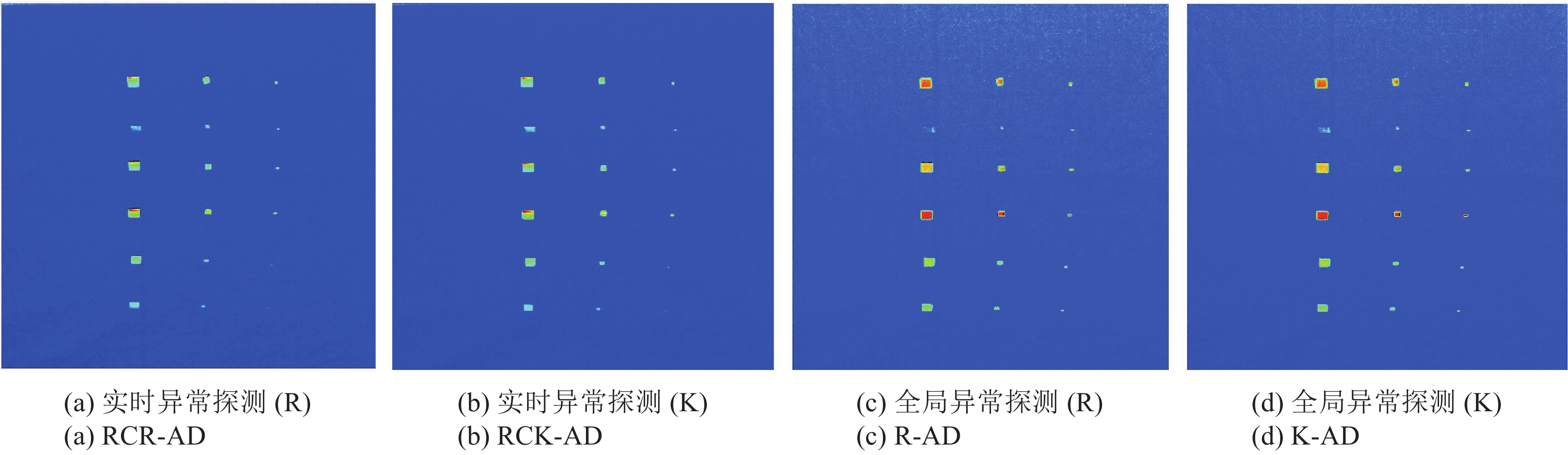
为进一步评价实时异常探测的精度,利用全局异常探测器(R-AD,K-AD)进行测试,图5为4种探测器(RCR-AD,RCK-AD,R-AD和K-AD)最终的探测结果灰度图。
4.3 探测精度评价
从图3和图4知,在RCR-AD和RCK-AD进行实时异常探过程中,异常目标出现之前,探测结果伪彩色图各像元强度值对比度较小;当第一个异常像元出现时,图像背景立即变暗,而异常像元则高亮显示;在所有6行目标中,第2行的异常响应最弱,与背景对比度最小。通过计算光谱相关系数,6种目标与背景之间的光谱相关性分别为0.898 (PRed)、0.962 (PBla)、0.873 (PBlu)、0.543 (PYel)、0.904 (FLGr)、0.919 (FDGr),可见第2行黑色纸质目标(PBla)与背景相关性最大,相对于背景而言,异常程度最低。因此,第2行目标在该场景中可理解为弱信号异常目标,而其他5行目标的信号强度则较大。
进一步观察发现,图5所示4种探测器的最终探测结果灰度图中,全局性异常探测器(R-AD,K-AD)均无法提取出第2行弱信号目标,而实时异常探测器(RCR-AD,RCK-AD)在渐进式处理过程中能够有效识别出该异常信号,防止其被后续探测到的强信号压制而无法识别。
利用图2(b)地面验证数据,采用3维接收器曲线(3D-ROC)(Chang,2013)对4种探测器的探测精度进行定量分析。首先将图5探测结果图的灰度归一化至0—1,在0—1范围内变换决策阈值τ,可将该探测结果图二值化为目标和背景,结合图2(b)地面验证数据,可得到特定阈值τ所对应的探测率PD,虚警率PF。因此,通过变化决策阈值τ,将得到一组(τ,PF,PD)用于生成3D-ROC。进一步地,从3D-ROC中可提取出3条2维ROC (2D-ROC),即2D-ROC (PD,PF)、2D-ROC (τ,PD)、2D-ROC (τ,PF)。
3D-ROC能够提供探测率PD和虚警率PF随决策阈值τ的变化趋势。此外,由于实际应用中异常探测为非监督过程,异常目标的识别主要依赖于对探测结果图的目视判断,因此,背景的压制效果对异常目标的决策影响较大(Chen 等,2014)。在这种情况下,2D-ROC (τ,PF)可以提供背景压制随τ的变化而变化的信息,而2D-ROC (τ,PD)则体现了探测率与决策阈值的变化关系。
图6为4种探测器(RCR-AD,RCK-AD,R-AD和K-AD)的ROC曲线图。为进一步定量化评价FISS数据的探测精度,表1为不同探测器的ROC曲线下面积AUC,探测性能最优的值为阴影显示,其中,A(τ,PD)和A(PF,PD)越大,或A(τ,PF)越小,探测精度越高,该异常探测器的性能越好。
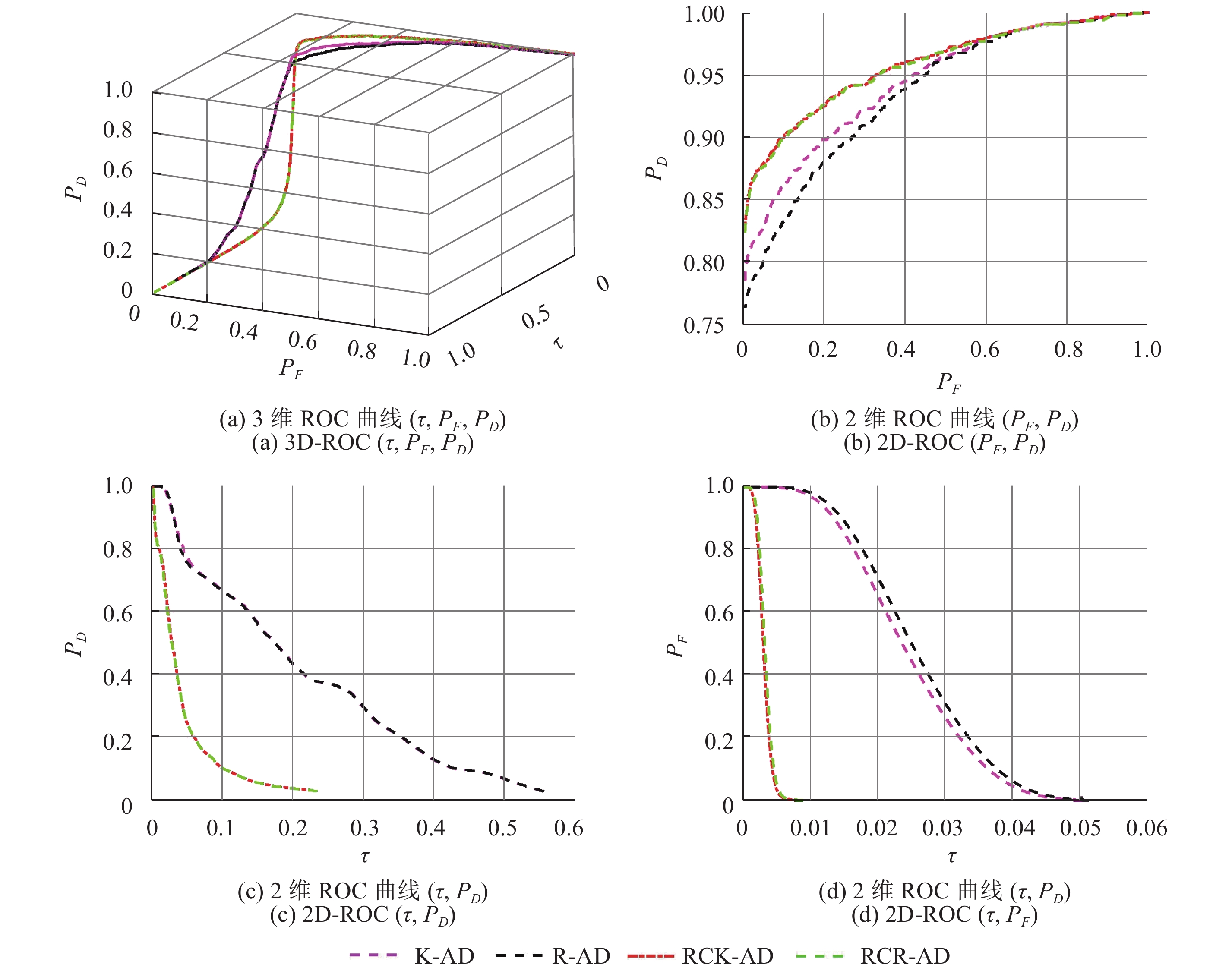
表 1 4种异常探测器所对应2D-ROC的AUC值
Table 1 Values of the AUC for each 2D-ROC
| Algorithm | RCK-AD | RCR-AD | K-AD | R-AD |
| A(PF, PD) | 0.9581 | 0.9573 | 0.9444 | 0.9362 |
| A(τ, PD) | 0.0490 | 0.0488 | 0.2102 | 0.2100 |
| A(τ, PF) | 0.0030 | 0.0032 | 0.0243 | 0.0256 |
从图6及表1可得出以下结论:(1) 由A(τ,PF)可知,实时异常探测器相较于全局性异常探测器而言,其背景压制更强,但是前者探测率A(τ,PD)比后者低,过度的背景压制易导致较低的探测率。(2) 虽然全局性异常探测器(R-AD,K-AD)具有较低的A(PF,PD),但其A(τ,PD)高于实时异常探测器(RCR-AD,RCK-AD)。因此,A(PF,PD)并非与A(τ,PD)正相关,仅利用传统的2D-ROC并不能有效地评价一个异常探测算法的探测性能。而3D-ROC能够从探测率、虚警率、背景压制等多方面综合评价一个探测器的性能。
4.4 算法时效性分析
算法时效性是衡量实时异常探测性能最重要的指标之一。为验证本研究所提出的实时异常探测器(RCR-AD,RCK-AD)的计算性能,对比分析了目前广泛使用的实时处理算法的计算性能并进行实验测试,主要包括基于背景统计矩阵QR分解的方法(QRR-AD、QRK-AD)(Chang 等,2001;Chang和Hsueh,2006;Hsueh,2007;Du和Zhang,2011;Molero 等,2013);基于Woodbury引理递归更新背景统计量的方法(WR-AD、WK-AD)(Du和Nekovei,2009;Acito 等,2011;Rossi 等,2012;Chen 等,2014;Rossi 等,2014;Chang 等,2015)。
基于Woodbury引理直接计算背景自相关矩阵的逆矩阵,其递归更新公式为
|
${{{R}}^{ - 1}}\left( n \right) = {{{\tilde{{R}}}}^{ - 1}}\left( {n - 1} \right) - \frac{{\left[ {{{{\tilde{{R}}}}^{ - 1}}\left( {n - 1} \right){{{\tilde{{r}}}}_n}} \right]\left[ {{\tilde{{r}}}_n^{\rm{T}}{{{\tilde{{R}}}}^{ - 1}}\left( {n - 1} \right)} \right]}}{{1 + {\tilde{{r}}}_n^{\rm{T}}{{{\tilde{{R}}}}^{ - 1}}\left( {n - 1} \right){{{\tilde{{r}}}}_n}}}$
|
(17) |
式中,
根据式(17),计算
基于背景自相关矩阵QR分解的方法,其步骤为:(1)对背景自相关矩阵R(n–1)进行QR分解
表2为上述各实时异常探测算法的理论时间复杂度,与本文所提出算法进行时效性对比分析。
表 2 理论时间复杂度
Table 2 Theoretical computational complexity
| 算法 | 时间复杂度/flops |
| RCR-AD | 3.5B2 |
| QRR-AD | 2B3+5B2 |
| WR-AD | 8B2 |
| RCK-AD | 6B2 |
| QRK-AD | 2B3+7B2 |
| WK-AD | 13B2 |
对上述各算法分别进行仿真实验测试。表3为各算法实时处理单个像元、整行像元的平均时间,及处理完整幅图像所花费的时间。可以看出,基于QR分解的实时处理算法涉及时间复杂度为O(B3),虽然避免了背景统计矩阵的求逆运算,但计算代价巨大;而基于Woodbury矩阵引理的方法需求解高维背景统计矩阵的逆,易造成数值不稳定(Stewart,1998;Seeger,2004),且由于其多次矩阵操作,涉及时间复杂度依然较高。本文所提出的基于Cholesky分解因子一阶修正的实时处理方法所需时间复杂度最低,能够在恒定且最短时间内输出当前时刻所获取像元的异常响应值,有效提高实时高光谱异常探测器的计算性能。
表 3 各实时处理算法处理单个像元、单行像元的平均时间以及处理完成整幅数据所需的时间
Table 3 Average computing time per pixel/line and the total time cost for the entire dataset using different real-time processing algorithms
| 算法 | 单个像元/s | 整行像元/s | 整幅图像/s |
| RCK-AD | 0.00092 | 0.42 | 189.9 |
| QRK-AD | 0.14221 | 65.98 | 29495.1 |
| WK-AD | 0.00280 | 1.30 | 580.4 |
| RCR-AD | 0.00056 | 0.26 | 115.1 |
| QRR-AD | 0.14127 | 65.55 | 29301.4 |
| WR-AD | 0.00207 | 0.96 | 428.8 |
5 结 论
本文提出一种基于Cholesky分解一阶修正的逐像元实时高光谱异常探测算法,定量讨论了算法的计算性能与探测精度,利用地面光谱成像辐射测量系统FISS所采集的室内高光谱数据进行仿真实时处理,得出以下结论:
(1) 通过对背景统计矩阵的Cholesky分解因子进行一阶修正,可快速更新下一时刻背景统计信息。结合下三角线性系统求解过程,实时处理时间缩短为基于QR分解算法的0.4%—0.65%,或基于Woodbury矩阵引理算法的27%—33%,且数值稳定性得以保持。
(2) 实时处理有助于观察背景压制效果的实时变化,防止弱异常信号被后续强信号所压制;另外,3D-ROC曲线有助于从背景压制、探测率、虚警率等方面综合评价探测器的性能。
本文所提出的实时高光谱异常探测算法在保持数值稳定性以及探测精度的前提下,有效提高实时处理的速度。但本文算法仅进行了计算机仿真实验,未利用机载高光谱成像仪进行真实场景下的实时处理测试,下一步将着重于无人机机载实时高光谱异常探测系统的研究。
参考文献(References)
-
Acito N, Matteoli S, Diani M and Corsini G. 2011. Complexity-aware algorithm architecture for real-time enhancement of local anomalies in hyperspectral images. Journal of Real-Time Image Processing, 8 (1): 53–68. [DOI: 10.1007/s11554-011-0205-x]
-
Bojanczyk A W, Brent R, Van Dooren P and De Hoog F. 1987. A note on downdating the Cholesky factorization. SIAM Journal on Scientific and Statistical Computing, 8 (3): 210–221. [DOI: 10.1137/0908031]
-
Chang C I. 2003. Hyperspectral Imaging: Techniques for Spectral Detection and Classification. New York: Springer [DOI: 10.1007/978-1-4419-9170-6]
-
Chang C I. 2013. Hyperspectral Data Processing: Algorithm Design and Analysis. Hoboken, NJ, USA: John Wiley and Sons [DOI: 10.1002/9781118269787]
-
Chang C I. 2016. Real-time Progressive Hyperspectral Image Processing: Endmember Finding and Anomaly Detection. New York: Springer [DOI: 10.1007/978-1-4419-6187-7]
-
Chang C I and Chiang S S. 2002. Anomaly detection and classification for hyperspectral imagery. IEEE Transactions on Geoscience and Remote Sensing, 40 (6): 1314–1325. [DOI: 10.1109/TGRS.2002.800280]
-
Chang C I and Hsueh M. 2006. Characterization of anomaly detection in hyperspectral imagery. Sensor Review, 26 (2): 137–146. [DOI: 10.1108/02602280610652730]
-
Chang C I, Li H C, Song M P, Liu C H and Zhang L F. 2015. Real-time constrained energy minimization for subpixel detection. IEEE Journal of Selected Topics in Applied Earth Observations and Remote Sensing, 8 (6): 2545–2559. [DOI: 10.1109/jstars.2015.2425417]
-
Chang C I, Ren H and Chiang S S. 2001. Real-time processing algorithms for target detection and classification in hyperspectral imagery. IEEE Transactions on Geoscience and Remote Sensing, 39 (4): 760–768. [DOI: 10.1109/36.917889]
-
Chen S Y, Wang Y L, Wu C C, Liu C H and Chang C I. 2014. Real-time causal processing of anomaly detection for hyperspectral imagery. IEEE Transactions on Aerospace and Electronic Systems, 50 (2): 1511–1534. [DOI: 10.1109/taes.2014.130065]
-
Du B and Zhang L P. 2011. Random-selection-based anomaly detector for hyperspectral imagery. IEEE Transactions on Geoscience and Remote Sensing, 49 (5): 1578–1589. [DOI: 10.1109/TGRS.2010.2081677]
-
Du Q and Nekovei R. 2009. Fast real-time onboard processing of hyperspectral imagery for detection and classification. Journal of Real-Time Image Processing, 4 (3): 273–286. [DOI: 10.1007/s11554-008-0106-9]
-
Gill P E, Golub G H, Murray W and Saunders M A. 1974. Methods for modifying matrix factorizations. Mathematics of Computation, 28 (126): 505–535. [DOI: 10.1090/S0025-5718-1974-0343558-6]
-
Golub G H and Van Loan C F. 2012. Matrix Computations. Baltimore: JHU Press [DOI: 10.1137/1032141]
-
Guo W J, Zeng X R, Zhao B W, Ming X, Zhang G F and Lv Q B. 2014. Multi-DSP parallel processing technique of hyperspectral RX anomaly detection. Spectroscopy and Spectral Analysis, 34 (5): 1383–1387. [DOI: 10.3964/j.issn.1000-0593(2014)05-1383-05] ( 郭文记, 曾晓茹, 赵宝玮, 明星, 张桂峰, 吕群波. 2014. 高光谱RX异常检测的多DSP并行化处理技术. 光谱学与光谱分析, 34 (5): 1383–1387. [DOI: 10.3964/j.issn.1000-0593(2014)05-1383-05] )
-
Hsueh M. 2007. Reconfigurable Computing for Algorithms in Hyperspectral Image Processing. Baltimore: University of Maryland, Baltimore County
-
Molero J M, Garzón E M, García I and Plaza A. 2013. Analysis and optimizations of global and local versions of the RX algorithm for anomaly detection in hyperspectral data. IEEE Journal of Selected Topics in Applied Earth Observations and Remote Sensing, 6 (2): 801–814. [DOI: 10.1109/JSTARS.2013.2238609]
-
Paz A and Plaza A. 2010. Clusters versus GPUs for parallel target and anomaly detection in hyperspectral images. Eurasip Journal on Advances in Signal Processing, 2010 : 915639 [DOI: 10.1155/2010/915639]
-
Press W H, Teukolsky S A, Vetterling W T and Flannery B P. 2007. Numerical Recipes 3rd Edition: the Art of Scientific Computing. 3rd ed. Cambridge: Cambridge University Press [DOI: 10.1145/1874391.187410]
-
Reed I S and Yu X. 1990. Adaptive multiple-band cfar detection of an optical pattern with unknown spectral distribution. IEEE Transactions on Acoustics, Speech, and Signal Processing, 38 (10): 1760–1770. [DOI: 10.1109/29.60107]
-
Rossi A, Acito N, Diani M and Corsini G. 2012. Computationally efficient strategies to perform anomaly detection in hyperspectral images//Proceedings of SPIE 8537, Image and Signal Processing for Remote Sensing XVIII. Edinburgh, United Kingdom: SPIE: 85370H [DOI: 10.1117/12.973686]
-
Rossi A, Acito N, Diani M and Corsini G. 2014. RX architectures for real-time anomaly detection in hyperspectral images. Journal of Real-Time Image Processing, 9 (3): 503–517. [DOI: 10.1007/s11554-012-0292-3]
-
Seeger M. 2004. Low rank updates for the Cholesky decomposition. No. EPREPORT-161468. 2004.
-
Stewart G W. 1998. Matrix Algorithms: Volume 1: Basic Decompositions. Philadelphia: Society for Industrial and Applied Mathematics [DOI: 10-1137/19781611971408]
-
Zhao B W, Xiang L B, Lv Q B, Zhang G F, Zeng X R and Guo W J. 2014. Parallel RX algorithm implementation based on the FPGA and multi-DSP system. Journal of Xidian University, 41 (3): 152–156. [DOI: 10.3969/j.issn.1001-2400.2014.03.022] ( 赵宝玮, 相里斌, 吕群波, 张桂峰, 曾晓茹, 郭文记. 2014. FPGA和多DSP系统的并行RX探测算法. 西安电子科技大学学报(自然科学版), 41 (3): 152–156. [DOI: 10.3969/j.issn.1001-2400.2014.03.022] )
-
Zhao C H, Wang Y L and Li X H. 2015. A real-time anomaly detection algorithm for hyperspectral imagery based on causal processing. Journal of Infrared and Millimeter Waves, 34 (1): 114–121. [DOI: 10.3724/sp.j.1010.2015.00114] ( 赵春晖, 王玉磊, 李晓慧. 2015. 一种新型高光谱实时异常检测算法. 红外与毫米波学报, 34 (1): 114–121. [DOI: 10.3724/sp.j.1010.2015.00114] )