Solutions to Forced and Unforced Lin–Reissner–Tsien Equations for Transonic Gas Flows on Various Length Scales
Theaker Kyle A.1, Van Gorder Robert A.2, *
Department of Mathematics, University of Central Florida, Orlando, FL 32816-1364, USA
Mathematical Institute, University of Oxford, Andrew Wiles Building, Radcliffe Observatory Quarter, Woodstock Road, Oxford, OX2 6GG, United Kingdom


† Corresponding author. E-mail: Robert.VanGorder@maths.ox.ac.uk

Abstract
Abstract

The Lin–Reissner–Tsien equation is useful for studying transonic gas flows, and has appeared in both forced and unforced forms in the literature. Defining arbitrary spatial scalings, we are able to obtain a family of exact similarity solutions depending on one free parameter in addition to the model parameter holding the scalings. Numerical solutions compare favorably with the exact solutions in regions where the exact solutions are valid. Mixed wave-similarity solutions, which describe wave propagation in one variable and self-similar scaling of the entire solution, are also given, and we show that such solutions can only exist when the wave propagation is sufficiently slow. We also extend the Lin–Reissner–Tsien equation to have a forcing term, as such equations have entered the physics literature recently. We obtain both wave and self-similar solutions for the forced equations, and we are able to give conditions under which the force function allows for exact solutions. We then demonstrate how to obtain these exact solutions in both the traveling wave and self-similar cases. There results constitute new and potentially physically interesting exact solutions of the Lin–Reissner–Tsien equation and in particular suggest that the forced Lin–Reissner–Tsien equation warrants further study.

1 Introduction

The Lin–Reissner–Tsien equation in dimensional units reads

This equation is used to study transonic gas flows under the transonic approximation.[13] Here is the dimensional velocity potential, are dimensional spatial coordinates, and is the temporal coordinate. In Glazatov,[4] existence and uniqueness results of a certain class of solutions to the Lin–Reissner–Tsien equation are proven, subject to specific periodic boundary conditions. Recently, Ref. [5] considered exact and analytical solutions for the Lin–Reissner–Tsien equation (1). In particular, both steady and non-steady similarity solutions were considered. For some parameter values, exact solutions were obtained, while for more general parameter regimes, analytical solutions were found via Taylor series. Under some simplifications, those solutions recovered other more specific exact solutions of Refs. [68]. Numerical solutions were also employed in Ref. [5] in order to verify the accuracy of the analytical approximations.

For some applications, the equation

is considered, where represents a dimensional external electromagnetic or mass force term. This and related equations are studied in Bogdanov,[9] with qualitative results about plane transonic flows being found. Bibik[10] obtains numerical solutions and then discusses the physical relevance for such solutions.

In the present paper, we shall consider the Lin–Reissner–Tsien equation on various length scales. We first non-dimensionalize the equation in Sec. 2, and are able to show that all spatial length scales enter through a single composite parameter multiplying the nonlinear term. This is useful, as depending on the length scales of interest, the parameter may be large or small. In Sec. 3, we seek the generalize some of the results from Ref. [5]. We first obtain a slightly more general similarity solution. Then, we turn our attention to mixed wave-similarity solutions, which were not previously considered. Such solutions propagate as a wave in one spatial coordinate, while still exhibiting a global self-similarity. Next, in Sec. 4, we consider generalized Lin–Reissner–Tsien equations with forcing terms. Equations similar to (2) have been shown to admit similarity solutions which are relevant in the study of transonic gas flows (i.e. Ref. [11], and references therein). Therefore, in the context of applications, it makes sense to consider forced Lin–Reissner–Tsien equations. We obtain traveling wave solutions, and are able to show that there are non-trivial (in contrast to the fairly simple traveling wave solutions which exist for (1)). We then show that forced Lin–Reissner–Tsien equations can still admit similarity solutions. We determine the precise class of forcing terms which allow for similarity solutions, before obtaining solutions numerically. We also show that a more restricted class of forcing functions allows for the construction of exact self-similar solutions. Finally, we give concluding remarks in Sec. 5.

2 Non-Dimensionalization and Scaling Limits

Let us non-dimensionalize the Lin–Reissner–Tsien equation (1) by the change of variables

Here X, Y, T, U are constants holding the relative scales of each variable. As we are concerned with spatial scales, while temporal scales are less essential, we can pick the temporal scale to simplify the resulting non-dimensional equation, by taking . We find then that

where the composite parameter ϵ depends on the remaining length scales like

Therefore, the Lin–Reissner–Tsien equation is reduced to a single equation on non-dimensional scales which depends only on a single scaling group. The spatial length scales are then all encoded in the single parameter ϵ, and it is sufficient to study (4) in order to study (1) under any length scales.

If , then either or , and we have the small-x or large-y scale limit. In such a limit, taking yields

Introducing the new variables , we have

which is a two-dimensional wave equation, plus a small perturbation. As such, we expect solutions in the small-ϵ regime to behave like solutions to a 2D wave equation.

If , then either or , and we have the large-x or small-y scale limit. In this case, the equation reduces to

This implies that

in the large-ϵ regime.

3 Similarity and Wave-Similarity Solutions for the Lin–Reissner–Tsien Equation

We now turn our attention to obtaining solutions to the scaled the Lin–Reissner–Tsien equation (4).

3.1 Similarity Transformation

Let us take the similarity transformation used in Ref. [5],

We obtain from Eq. (4) the similarity ODE

where prime denotes differentiation with respect to the similarity variable, η. The equation becomes singular for , or, in the limit,. In this limit, (11) reduces to

Then, at such a singular point η = 1/2, the natural boundary condition would read

Hence, the boundary condition

shall be taken at η = 1/2. If we solve the linearized equation (12), we obtain

where A is a free parameter. Yet, for this solution, ϕ(0) = A. Hence, it makes sense to consider the additional boundary condition

We shall this be interested in solutions to the boundary value problem consisting of (11) subject to (14) and (16) for small positive ϵ.

3.2 Exact Solutions to the Similarity Problem

Here we obtain exact solutions to the similarity ODE (11). First, assume that

Then, placing this assumption into (11), we obtain the algebraic equation

from which we get the system

Leaving A fixed yet arbitrary, we can find B and C as such:

Thus,

Returning to physical coordinates, we have

The exact solution (
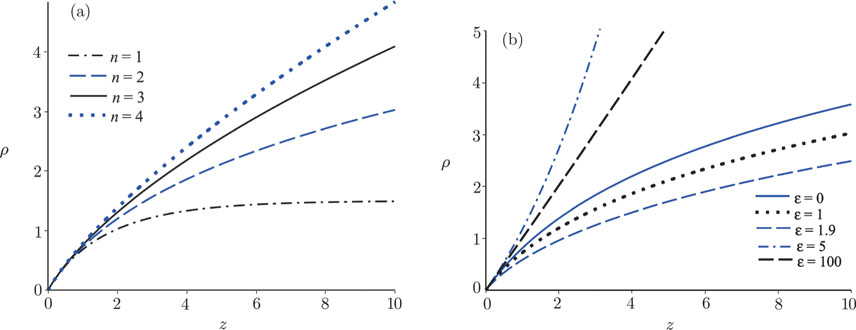
23) is the solution given in Eq. (37) of Ref. [5], with two modifications. First, the solution (23) is more general, in that it involves an arbitrary parameter . Second, the solution (23) also depends on the arbitrary scaling parameter . Therefore, we conclude that this solution is more general than that of Ref. [5].

3.3 Numerical Solutions to Eqs. (11), (14), (16)

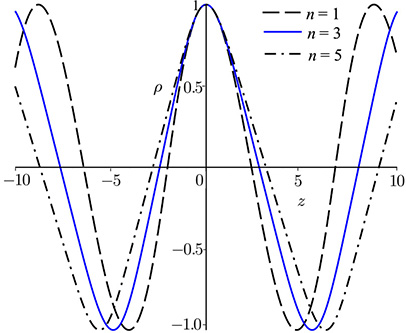
With one class of exact solutions obtained, we now turn our attention to numerical solutions of the boundary value problem given by the ODE (11) subject to boundary conditions of the form (14) and (16). Since we are primarily interested in the influence of the scaling parameter, ϵ, on the solutions, we shall take ϕ(0) = 1 for these simulations. We plot solutions in Fig. 1.

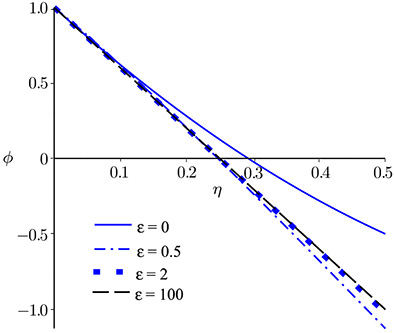
Fig. 1 Plot of the numerical solutions of the boundary value problem given by the ODE (11) subject to boundary conditions of the form (14) and (16), given that we fix the parameter A = 1. We plot the solutions for various values of ϵ, finding that for sufficiently large ϵ the solutions take on a linear appearance. This makes sense, as the linear solution is the only solution in the limit .
3.4 Mixed Wave-Similarity Transforms

Let us consider a wave variable along the x direction; that is to say, z = xct. Such solutions were not considered in Ref. [5] or elsewhere. Then (4) becomes

Consider a solution of the form ,. Then,

Placing these into Eq. (24) gives us

For this equation, we must have 2 + 2b = 0 and a + 2 + 3b = 0, which implies that a = 1 and b = −1. With these similarity parameters, we obtain

It is clear from the form of (27) that there will always be a constant solution,. Then, this solution gives the physical solution u(y, z) = Cy. One may easily verify that this is indeed a solution to (4).

To find a second solution, let us consider the transformation , which puts (27) into the form

In the limit where , we simply obtain for arbitrary constant . Integrating, we recover

Returning to physical variables, we have

In the more interesting case where ϵ is not negligible, and to make this case more tractable we make the change of variable

which gives us the ODE

This ODE permits an exact solution of the form

where W denotes the Lambert W function (which satisfies the implicit functional equation ) and is a constant. This then gives

We then integrate this equation over σ to recover f(σ),

The arbitrary constant must be picked so that a branch of the Lambert W function W actually exists, i.e.. Finally, transitioning back into physical coordinates, we obtain the exact solution to (4), which takes the form

Interestingly, the solution (36) does not always exist on . Indeed, we must have that

Therefore, the solution exists only for . If , then there will exist some region of the plane for which the solution fails to exist. Physically, this means that solutions of the type (36) have a maximum possible wave speed . At and beyond this critical value, the solutions will breakdown in finite time if the wave moves too fast () in the positive x direction.

To conclude this section, we give numerical plots of the solutions to Eq.‘(27) in Fig. 2.

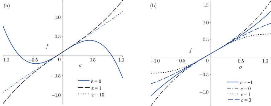
Fig. 2 Plot of the numerical solutions to (27) for (a) various values of ϵ for fixed wave speed c = 0.2 and (b) various values of the wave speed c for fixed ϵ = 0.5. The boundary conditions are fixed as f(0) = 0.1 and f′(0) = 1 for all plots.
4 Lin–Reissner–Tsien Equation with Forcing Terms

Next we consider the forced Lin–Reissner–Tsien equation

where F is a forcing term. Such equations are useful in the study of gas dynamics.[11]

4.1 F = F(u)

Let F = F(u). Consider a wave solution

Then, we obtain the ODE

where prime denotes differentiation with respect to z. Unlike the pure traveling wave case discussed in Ref. [5], the inclusion of the forcing function can lead to more complicated dynamics, in contrast to the case of no forcing, for which the pure traveling wave solutions are trivial.

If we multiply Eq. (40) by ρ′ and integrate, we obtain

where is the antiderivative of F(u).

For various values of the parameters, we may plot the phase portraits in order to understand the behavior of solutions to this equation. On the other hand, we may directly solve the ODE (40) numerically. We do so in Fig. 3.

Fig. 3 Plot of the numerical solutions to (40) given for various values of the power-law parameter n. The other parameters are fixed as b = c = 1, ϵ = 1, and α = 1, while boundary conditions are taken as ρ(0) = 1, ρ′(0) = 0. In order to obtain periodic solutions, we consider only odd n. The solutions do not vary strongly with ϵ, and the role of is to modify the period of the solutions. The structure of the solutions is most influenced by n. As n increases, the traveling wave solutions become more sharp and the period of oscillation decreases, although the amplitude remains the same.

In the special case were , so that the wave variable is , we have

which gives us

Suppose that the force scales with a power of u, say for some positive integer n and constant parameter α. Then, we obtain the implicit relation

4.2

Consider now the case where the forcing function depends on the derivatives of u, say . Under the assumption of a traveling wave solution (39), we find that

where by H(ρ′) we denote

Separating variables in Eq. (45) and integrating, we obtain an implicit relation for the function ρ′:

Consider the case where the force scales as a power of the first derivatives of u, so that we obtain for some positive integer n and constant parameter β. We then have three cases:

for n = 1,

for n = 2, and

for . If we are able to invert these relations, we may then obtain ρ′ as a function of z. Integrating that result would then permit us to recover ρ(z). This may also be done numerically, and we provide plots of the numerical solutions for various n and ϵ in Fig. 4.

Fig. 4 Plot of the numerical solutions to (45) given for various values of the power-law parameter n. The other parameters are fixed as b = c = 1 and β = 1, while boundary conditions are taken as ρ(0) = 0, ρ′(0) = 1. In (a) we fix ϵ = 1 and plot the solutions for various n. As n increases, the solutions uniformly increase in magnitude. In (b) we fix n = 2 and plot the solutions for various ϵ. For 0 < ϵ < 2, the solutions uniformly decrease in magnitude as ϵ increases. At ϵ = 2, the problem becomes singular, and for ϵ > 2 we then obtain a new type of solution branch. The curve starts out steep, and gradually decreases in slope as ϵ increases toward infinity.
4.3 Forms of F which Permit Similarity Solutions

As discussed in Ref. [11], it is possible to have self-similar solutions to equations arising in gas dynamics, even when there is a forcing term present within the governing equation. We seek to find a general form of F = F(x, y, t) which still allows for a similarity solution.

Due to the similarity transform (10), we should consider

where a, b, c, γ are constant parameters that would be selected based on the physical problem to be studied. Then, under the assumption (10), we find that (38) reduces to

The right hand side of (52) should take the form of a power of η, the similarity variable. Noting that , we should have a = k, b − 2 = −2 k, c + 3 = k. Then,

In other words, the permitted form of the force F is a power of the similarity variable, η, multiplied by a factor . Under such an assumption, we have that

We numerically solve (54) for various k, in order to determine the influence of ϵ for each of these cases. In Fig. 5, we plot numerical solutions to (54) in order to determine the influence of the strength of the forcing function on the solutions.

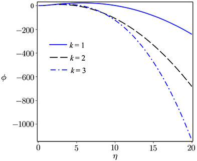
Fig. 5 Plot of the numerical solutions to (54) given for various values of the power-law parameter k. The other parameters are fixed as ϵ = 1 and γ = 1, while boundary conditions are taken as ρ(0) = 1, ρ′(0) = 0. As we increase k, the solutions uniformly decrease in value, more rapidly tending toward negative infinity as η becomes large.

In addition to numerical solutions, note that it is also possible to obtain exact solutions for the similarity problem (54). Along the lines of the earlier exact solution (17), we assume a polynomial solution

Here, the ’s are constants to be determined. If γ = 0, then the solution (55) will reduce to the exact solution (17), with m = 2 and both and determined as functions of the free parameter .

On the other hand, if , then the existence of an exact polynomial solution will depend on the power law parameter k. If a polynomial solution (55) does indeed exist, then the order of the left hand side of (54) with the proposed exact solution plugged in must match the order of the right hand side (which is simply k). If m = 0, 1, 2, 3, then the linear terms in (54) will dominate. However, if m > 3, then the nonlinear term will have order 2m − 3, which is greater than m for m > 3. So, if k = 0, 1, we pick m = 2, while if k = 3, we pick m = 3. It is less clear what to do when k = 2, since m = 2 results in no quadratic terms remaining on the left hand side of (54). While we omit a lengthy argument here, when k = 2, one may show that a polynomial solution would only exist for either complex-valued ϵ or complex-valued γ. However, if k > 3, then we must be more careful. If k = 4, observe that there is no integer m such that 2m − 3 = 4 (m = 1/2 in this case). Indeed, for k > 4, an exact polynomial solution (55) exists only when 2m − 3 = k has a positive integer root , i.e. k must be odd. The first few permitted values of k are k = 5 (for which m = 4), k = 7 (for which m = 5), and so on. For other integer values of k > 0, there are no exact polynomial solutions. Therefore, there are possible polynomial solutions provided the forcing function satisfies k = 0 or k a positive odd integer. For other values, numerical simulations can be used, but exact solutions in terms of polynomials are not forthcoming.

We explicitly calculate the first few exact solutions, finding that for k = 0 we have

for k = 1 we have

and for k = 3 we have

where

For k > 3, although solutions are theoretically possible due to order balances discussed above, when calculating the actual solutions we find that the equations for the coefficients in (55) will be over determined. This will result in complex coefficients or parameters, and hence such solutions should be neglected as they are non-physical. Therefore, the exact solutions above are the only polynomial solutions, and exact polynomial solutions fail to exist for k > 3. Meanwhile, note that we see something related in those exact solutions we can obtain. When k = 0 or k = 1, the system of equations for the coefficients is under-determined, meaning we always have a free parameter (for us, this is ). This is exactly why we had the free parameter A in the exact solution (17). When k = 3, the coefficients of the solution were uniquely determined, which is why the solution for k = 3 does not have a free parameter, but rather will only depend on system parameters ϵ and γ. Still, owing to the nonlinearity, the solution for k = 3 is not unique, with two solutions existing (depending on the ± root in the definition of ).

5 Conclusions

We have extended the results of Ref. [5] in several ways. First, we have found additional solutions to the Lin–Reissner–Tsien equation, including a somewhat more general similarity solution and new mixed wave-similarity solutions. We have also extended the Lin–Reissner–Tsien equation by considering a forcing term. Such forced equations are useful in the study of gas dynamics.[11] For the forced equation, we are able to study a variety of forcing functions, which permit either new wave or similarity solutions. Unlike for the standard Lin–Reissner–Tsien equation, the forced equation permits non-trivial wave solutions. It is interesting that, despite the added complexity due to the forcing term, the forced equation still permits similarity solutions, and for some cases can even still be solved exactly. We are able to determine precisely for which forcing functions exact polynomial solutions will exist. These results suggest that, while complicated, forced Lin–Reissner–Tsien equations can still be solved exactly under some circumstances. For all of the various solutions obtained, numerical simulations verify the behaviors observed in exact or perturbation solutions.

Many of the solutions only exist for certain parameters or parameter regimes. Therefore, some of the parameter values correspond to physically relevant solutions, while parameters for which there are no solution would correspond to a loss of validity of the transonic approximation, or more fundamentally, a breakdown of the transonic gas flow. In such a case, more complicated dynamics, such as turbulence, may arise, which is beyond the scope of the LRT equation. So, when there is a solution, this means that the physical parameters permit a “nice” solution to the transonic gas flow problem. The solutions in Subsec. 3.4 further depend on a wave speed, c. We find that left-moving waves (c < 0) are permitted at any velocity, while right-moving waves can propagate only with a velocity bounded like . For right-moving waves with higher velocity, the wave would likely become unstable and break apart, resulting in turbulence. Note that the break-up is local in nature, in the case of . This suggests that, give a specific wave speed, we can determine where in space the break-up of the wave solution under the transonic approximation may occur in time, given specific spatial coordinates.

The LRT equation with forcing term was also considered. While the precise form of forcing can be determined by the particular experiment at hand, we provide some examples to illustrate that solutions to forced LRT equations can exist. The form of the forcing term will strongly influence the dynamics of the LRT solutions. If the forcing function scales as a power of the unknown function, then we can expect periodic waves, with the frequency of the waves decreasing as the power of the function increases. Therefore, we have bounded, periodic transonic wave solutions for the gas in this regime. On the other hand, when the forcing function depends on one or more first derivatives of the unknown function, the transonic gas solutions are monotone increasing if we have traveling wave solutions. Therefore, the structure of the forcing term will strongly influence the behavior of traveling wave solutions.

Forced LRT equations also have solutions under a similarity transformation, assuming appropriate forcing term. In such a case, the solutions are highly sensitive to the strength of the nonlinearity in the forcing term. In this case, we also show that certain forcing functions, while theoretically possible, do not give closed-form similarity solutions. This again has to do with the fact that such poorly behaved forcing functions would likely cause breakdown of a solution over time, resulting in a transition to the turbulent regime.

The closed form solutions presented here cast light on when solutions to the LRT equations are possible. In other situations, solutions are not possible (or, not found), and this can indicate other behaviors, such as turbulence, which cannot be captured by the LRT model. Since the solutions have been non-dimensionalized, this means what solutions may be possible at some scales, while at other scales the solutions under the LRT transonic gas model will break down, giving way to turbulent gas dynamics. In particular, solutions always exist when ϵ = 0, and are found for small ϵ, as well. In terms of the space and time scales,. Then, when , hence solutions tend to always exist for large timescales (relative to the spatial scales). In contrast, the mixed wave-similarity solutions of Subsec. 3.4 are valid either for or , with very different solutions obtained for each case. The former solution can be viewed as the “large-time scale” solution, while the latter can be viewed as the “short-time scale” solution. Therefore, even when solutions are possible at all scales, there are often qualitative differences in the behaviors of the obtained solutions at disparate scales. All of these results will therefore inform us of how solutions should behave at different space or time scales. When coupled with the results for the forced LRT equation, these solutions may then serve as motivation for certain experiments on transonic gas dynamics under specific forcing terms.

Reference
[1] Lin C.C. Reissner E. Tsien H.S. J. Math Phys. 27 1948 220
[2] Ames W.F. Nucci W.N. J. Eng. Mech. 20 1985 18
[3] Kuz’min A.G. Ivanova A.V. Theor. Comput. Fluid Dyn. 18 2004 335
[4] Glazatov S.N. Mathematical Notes 87 2010 130
[5] Hausserman J. Vajravelu K. Van Gorder R.A. Appl. Math. Mech. -Engl. Ed. 32 2011 1447
[6] Titov S.S. A Method Finite-Dimensional Rings for Solving Nonlinear Equations of Mathematical Physics, [in Russian] Aerodynamics Ivanova T.P. Saratov University Saratov 1988 104
[7] Svirshchevskii S.R. Phys. Lett. A 199 1995 344
[8] Polyanin A. D. Zaitsev V.F. Handbook of Nonlinear Partial Differential Equations Chapman & Hall/CRC Boca Raton 2004
[9] Bogdanov A.N. Duesperov V.N. J. Appl. Math. Mech. 72 2008 33
[10] Bibik Yu.V. Duesperov V.N. Popov S.P. Fluid Dynamics 40 2005 315
[11] Bellout H. Vajravelu K. Van Gorder R.A. Quart. Appl. Math. 73 2015 379