

|
收稿日期: 2018-01-23
基金项目: 国家自然科学基金(编号:61501407,61772425,61701415);河南省科技创新杰出人才(编号:184200510015);河南省高校科技创新团队(编号:19IRTSTHN013);郑州轻工业学院博士基金(编号:2014BSJJ016)
第一作者简介: 钱晓亮,1982年生,男,讲师,研究方向为模式识别与人工智能、遥感图像场景分类与目标检测。E-mail:qxl_sunshine@163.com
通信作者简介: 姜利英,1981年生,女,教授,研究方向为数字图像处理、智能检测技术。E-mail:jiangliying@zzuli.edu.cn
中图分类号: TP753
文献标识码: A
|
摘要
高分辨率遥感图像场景分类方法主要涉及两个环节:特征提取以及特征分类,分类器的设计已经相对成熟,当前工作的重点是特征提取策略的研究。为了进一步推动特征提取策略的研究,将特征提取策略对高分辨率遥感图像场景分类性能的影响进行了定性和定量评估。首先,回顾了高分辨率遥感图像场景分类的发展历程;然后,对现有高分辨率遥感图像场景分类方法的特征提取策略进行分类总结,并从理论上将各类特征提取策略对场景分类性能的影响进行定性评估;最后,在3个规模较大的数据集上对多种特征提取策略进行实验对比,将不同特征提取策略对场景分类性能的影响和各数据集的复杂度进行定量评估。
关键词
高分辨率, 场景分类, 特征提取策略, 手工特征, 数据驱动特征, 深度学习
Abstract
Remote sensing image scene classification aims to tag remote sensing images with semantic categories according to the content of the image and is important in disaster monitoring, environmental detection, and urban planning. Scene classification results can provide valuable information about object recognition and image retrieval and can effectively improve the performance of image interpretation. The general process of remote sensing image scene classification mainly consists of feature extraction and scene classification based on image features. Given that the design of classifiers is relatively mature, this work focuses on feature extraction strategy. The influence of various strategies on the performance of scene classification is short of unified evaluation, which limits its development. The effect of various feature extraction strategies on the performance of high-resolution remote sensing image scene classification is evaluated in this study. In the second section of this paper, existing feature extraction strategies are divided into two categories: (1) hand-designed and (2) data-driven feature extraction. Hand-designed features, such as Color Histograms (CH) and Scale Invariant Feature Transform (SIFT), provide the primary description of images and are presented in the early period. Further abstract description of the images is introduced by coding of hand-designed features, such as Bag of Visual Words (BoVW) and has higher classification accuracy than hand-designed features. However, these feature extraction strategies generally suffer from poor generalization capability due to specific requirements for designing. Furthermore, hand-designed features require significant domain knowledge. By contrast, data-driven features can directly learn powerful features from a large number of sample images and are generally divided into shallow and deep learning features. Shallow learning feature extraction mainly involves Principal Component Analysis (PCA), Independent Component Analysis (ICA), and sparse coding algorithms. Typical deep learning feature extraction strategies include stacked autoencoder (SAE), Deep Belief Network (DBN), and Convolutional Neural Network (CNN). Compared with deep learning models, shallow learning models can be regarded as a neural network with a single hidden layer and thus cannot capture high-level semantic features. The superiority of deep learning features is obvious when dealing with complex scene classification. Furthermore, CNN-based features exhibit improved performance compared with SAE- and DBN-based features because the one-dimensional structure of SAE and DBN destroys the spatial information of images. In the third section of this paper, 29 feature descriptors are quantitatively compared in UC Merced, AID, and NWPU RESISC-45 datasets and eight combinations of feature descriptors are quantitatively compared in the NWPU RESISC-45 dataset. The effect of different feature extraction strategies on the performance of scene classification and the complexity of each dataset are evaluated through quantitative comparison. The experimental results are as follows. (1) The classification accuracy and stability of hand-designed features is poor, however the efficiency of most features is satisfactory and can attain better performance by combining with other types of features. (2) Among all feature extraction strategies, the coding of hand-designed features possesses moderate levels of classification accuracy, efficiency, and stability. (3) The classification accuracy and stability of data-driven features are best, but most of them have low efficiency. (4) AlexNet, a deep learning model with few layers, exhibits the best comprehensive performance and is suitable for occasions that require high classification accuracy, efficiency, and stability. (5) Some scene classes belonging to land use type are easy to be confused because of similar landmark buildings or sites. Moreover, some scene classes belonging to land cover type are easy to be confused because of their similar geomorphologic features. (6) The recently proposed NWPU RESISC-45 dataset is more complex than the other datasets and is more challenging for scene classification algorithms. Finally, the summary and conclusion of this paper are presented, and the discussion of future development is provided. On the one hand, combining prior knowledge introduced by hand-designed features with the CNN model may be one of the future development directions. On the other hand, introducing Generative Adversarial Networks (GAN) into CNN training may be a research hotspot in the future. In addition, remote sensing parameters, such as NDVI and NDWI, and multi-spectral information can be integrated with current feature extraction strategies for practical applications.
Key words
high-resolution, scene classification, feature extraction strategy, hand-designed features, data driven features, deep learning
1 前 言
近年来,随着遥感成像技术的不断发展,遥感图像的分辨率(空间分辨率、光谱分辨率、辐射分辨率和时间分辨率)和质量有了很大地提高,遥感图像分类任务也随之发生变化,目前该领域的学术研究主要集中于高分辨率遥感图像场景分类和高光谱遥感图像分类这两类。高分辨率遥感图像的空间分辨率较高,而光谱信息相对匮乏,因此高分辨率遥感图像场景分类主要是利用图像的空间信息和少量的光谱信息来识别给定遥感图像的场景类别(Gong 等,2018;Han 等,2017;Liu 等,2018;Wang 等,2017b;Zhao 等,2016b;Zhu 等,2017),常用的公开数据集一般包含多幅属于不同场景类别的高分辨率遥感图像(一般只包含3个光谱通道),1幅图像对应1个类别标签,图1(a)所示即为高分辨率遥感图像场景分类的示例。高光谱遥感图像包含丰富的光谱信息,但是空间分辨率相对较低,因此高光谱遥感图像分类主要是利用图像丰富的光谱信息和少量的空间信息对一幅图像的像元进行区域分类并识别各区域的类别(Guo 等,2016;Kasapoglu和Ersoy,2007;Wan 等,2015;Xue 等,2017;Zhang 等,2012),常用的公开数据集一般只包含1幅含有多个地物类别的高光谱遥感图像,图像中的一片像元区域对应1个类别标签,图1(b)所示即为高光谱遥感图像分类的示例。


高分辨率遥感图像场景分类能够有效地辨别土地利用情况,其结果也可以为目标识别和检索任务提供重要的参考信息,有效提高图像解译的性能(祁昆仑,2017),在自然灾害监测、环境检测、交通监管、武器制导和城市规划等应用方面具有重要的意义(许夙晖 等,2016)。因此,高分辨率遥感图像场景分类一直是遥感领域的研究热点。
20世纪70年代,卫星遥感图像的空间分辨率普遍较低,遥感图像场景分类方法的研究主要集中在像素层面(Tuia 等,2009, 2011),即对图像中的像素进行统计研究。由于单个像素丢失了语义信息且遥感图像的空间分辨率有了很大提高,所以基于像素层面的方法已经不能满足辨别遥感图像场景类别的任务需求。21世纪初,人们普遍认为在物体层面的方法更有研究意义,其中的物体指在图像中能够辨别的语义实体或者场景部分。相比于像素层面,物体层面的研究方法对图像的描述更高级,将来学者们的研究也会一直集中在物体层面(Blaschke, 2003, 2010;Gao 等,2006)。
虽然物体层面的研究方法在土地类型的分类任务上表现优秀,但是在语义层面上对遥感图像的意义以及内容的理解还差强人意。随着机器学习理论的快速发展,近些年提出了一些在语义层面的遥感图像场景分类的方法(Liu 等,2016;Zhao 等,2016a, 2016b, 2016c),能够很好地分别出图像的语义类别。
尽管新的场景分类方法不断涌现,但是在场景分类方法的评估上缺乏针对性。事实上,特征描述符对场景分类的性能影响很大,因此特征提取策略的研究一直是本领域的重点。然而,现有工作大多是对场景分类方法的整体性能进行评估,且实验对比大多是在不同数据集上进行(一般不对外开放代码),缺乏特征提取策略对场景分类性能影响的统一评估,不利于特征提取策略的进一步研究。
针对上述问题,本文从理论分析和实验对比两个方面,将特征提取策略对高分辨率遥感图像场景分类性能的影响进行了定性和定量评估。本文的主要贡献为:(1)对现有的高分辨率遥感图像场景分类方法的特征提取策略进行分类总结,并从理论上将各类特征提取策略对场景分类性能的影响进行定性评估;(2)在3个高分辨率遥感图像数据集(包含两个场景类别数不低于30类的大规模数据集)上进行实验对比,通过多个评价指标将特征提取策略对高分辨率遥感图像场景分类性能的影响进行定量评估;(3)将所有特征提取策略在3个数据集上的实验结果进行综合分析,对数据集的复杂度进行评估与分析。
2 高分辨率遥感图像场景分类方法特征提取策略的总结与定性评估
高分辨率遥感图像场景分类的流程如图2所示。首先对输入图像进行特征提取,然后分类器利用图像特征进行分类得到最终结果。其中,分类器的研究已经相对成熟,当前工作的重点之一就是特征提取策略的研究。现有高分辨率遥感图像场景分类方法的特征提取策略可大致分为两类:(1)手工特征的提取;(2)数据驱动特征的提取。

2.1 手工特征
高分辨率遥感图像场景分类方法常用的手工特征包含:颜色直方图、纹理特征、GIST和SIFT等。在所有的手工特征中,颜色直方图CH(Color Histograms)(Swain和Ballard,1991)的应用最为广泛,CH特征包含图像中的颜色分布信息,已有多种方法将CH应用到场景分类中(Li 等,2010;Penatti 等,2015;dos Santos 等,2010;Shyu 等,2007)。纹理特征可以提供图像局部区域内像素灰度级的空间分布信息,本领域有多种提取纹理特征的方法,如共生矩阵GLCM(Gray Level Co-occurrence Matrix)(Haralick 等,1973)、Gabor滤波器(Jain 等,1997)和局部二进制模式LBPs(Local Binary Patterns)(Ojala,1996)等,采用纹理特征的场景分类工作有Aptoula(2014)、Bhagavathy和Manjunath(2006)和Newsam等(2004)等。SIFT特征(Lowe,2004)是提取图像关键点的局部特征,有大量场景分类方法使用SIFT特征(Avramović和Risojević,2016;Luo 等,2013;Yang和Newsam,2008)。GIST特征通过5种空间包络模型获取的特征描述可以表示场景的主要空间结构,采用GIST特征(Oliva和Torralba,2001)的场景分类方法有Avramović和Risojević(2016)和Risojević等(2011)等。
很多高分辨率遥感图像场景分类方法将手工特征进行编码,以此作为图像的特征表示,以BoVW模型(Bag of Visual Words)(Li和Perona,2005)为典型代表。BoVW的主要思想是先对图像提取局部手工特征,然后对这些特征进行聚类得到一个“词袋”,最后利用“词袋”对图像进行编码得到一个直方图,以此作为图像的特征描述。它的提出使得场景分类的研究产生了巨大飞跃,有大量场景分类方法(Chen 等,2011;Hu 等,2015a, 2015b;Sridharan和Cheriyadat,2015;Zhao 等,2014)采用BoVW或BoVW的改进模型。围绕BoVW模型的改进工作主要包括SPM(Spatial Pyramid Matching)、(Yang和Newsam,2010)ScSPM(Sparse Coding Spatial Pyramid Matching)(Yang 等,2009)、LLC(Locality-constrained Linear Coding)(Wang 等,2010)、pLSA(probabilistic Latent Semantic Analysis)(Negrel 等,2014)、LDA(Latent Dirichlet Allocation)(Blei 等,2003)、IFK(Improving the Fisher Kernel)(Perronnin 等,2010)和VLAD(Vector of Locally Aggregated Descriptors)(Jégou 等,2012)等。
2.2 数据驱动特征
数据驱动特征可分为浅层学习特征和深度学习特征。浅层特征提取是相对深度特征提取而言,可以视作一种单隐层的神经网络特征提取方法。
2.2.1 浅层学习特征
高分辨率遥感图像场景分类方法常用的浅层学习特征主要包括主成分分析PCA(Priciple Component Analysis)(Jolliffe,2005)、独立成分分析ICA(Independent Component Analysis)(Comon和Pierre,1994)和稀疏编码(Sparse Coding)(Olshausen和Field,1997)等。
PCA是一种早期的无监督特征提取算法,将PCA运用到遥感领域的场景分类方法有Chaib等人(2016a, 2016b)和Wang等人(2017a)的方法,它通过一个转换矩阵来获取图像的特征描述,该特征可以通过较少的数据量包含图像中的主要信息。ICA的基本思想是从一组混合的非高斯模型信号中分离出独立信号,即用一组相互独立的基向量对其他信号进行表示,采用ICA来提取特征的场景分类方法有Cousin等人(2011),Du等人(2006)和Karoui等人(2009)等方法。Sparse Coding是通过大量的训练样本得到一组超完备的基向量,并以此来对图像进行编码,要求只有少部分的编码系数不为0,以编码系数(Cheriyadat,2014;Sheng 等,2012)或重构误差(Han 等,2014;Mekhalfi 等,2015)作为最终的特征表示,Dai和Yang(2011)、Mekhalfi等人(2015)和Zheng等人(2013)将此类特征应用到遥感图像场景分类中。
2.2.2 深度学习特征
深度学习特征可大致分为两类,一类基于“1维”深度神经网络DNN(Deep Neural Network)来提取特征,即:输入为1维矢量;另一类采用“2维”DNN,即:输入为2维图像(或是3通道的彩色图像),前者的典型代表是基于深度置信网络DBN(Deep Belief Network)(Hinton 等,2006)和堆叠自编码器SAE(Stacked Autoencoder)(Vincent 等,2010)的场景分类方法,后者的典型代表是基于卷积神经网络CNN(Convolutional Neural Network)(Krizhevsky 等,2012)的场景分类方法。
DBN是一个概率生成模型,由一系列受限玻尔兹曼机RBM(Restricted Boltzmann Machine)组成,采用非监督贪婪逐层训练算法(Bengio 等,2007)进行预训练。有多种场景分类方法(Chen 等,2015, 2016;Hou 等,2015;Zhong 等,2016, 2017)采用DBN来提取特征。自编码器(Hinton和Salakhutdinov,2006)是只有一层隐藏节点且输入和输出具有相同节点数的对称神经网络,其目的是使输出尽量逼近输入。SAE则是由多个自编码器连接而成的,即前一个自编码器的输出作为后一个自编码器的输入。采用SAE的工作主要有Du等人(2017)和Yao等人(2016)等研究。
CNN一经提出,便以其强大的特征提取能力成为本领域的研究热点,它采用“2维”卷积的形式对图像进行了多层的抽象表达。目前有众多基于CNN的场景分类工作,如Hu等人(2015a)、Luus等人(2015)、Penatti等人(2015)、Zhang等人(2016)、Zhao和Du(2016)和Zhong(2016)等研究。自从AlexNet(Krizhevsky 等,2012)获得成功后,多种基于卷积神经网络的方法也被陆续提出,如Overfeat(Sermanet 等,2014)、VGGNet(Simonyan和Zisserman,2014)、CaffeNet(Jia 等,2014)、GoogLeNet(Szegedy 等,2015)、SPPNet(He 等,2014)和ResNet(He 等,2016)等。此外,还有一些方法将CNN与其他的方法模型进行了结合,如Hu等人(2015a)分别从不同深度的CNN全连接层提取图像特征,并将其作为局部特征,然后结合特征编码模型对这些局部特征进行编码得出全局特征,使用的编码模型有BoVW和IFK等。Cheng等人(2017b)将图像块输入CNN得出图像的局部特征,然后用K-means聚类得到词典,再结合BoVW模型进行编码得到图像的全局特征。
2.3 特征提取策略对场景分类性能影响的定性评估
2.3.1 手工特征对场景分类性能影响的定性评估
在手工特征中,CH特征对图像本身的尺寸、方向等信息的依赖性小,对光照变化以及量化误差比较敏感,但是由于不包含图像的空间信息,因此基于CH特征直接分类的方法很难区分具有相同颜色但颜色分布不同的场景图像。纹理特征可以体现遥感图像中由地物重复排列而造成的灰度值规律分布,所以基于纹理特征直接分类的方法能很好地辨别纹理场景图像,但是不易区分纹理特征不丰富的场景图像。SIFT及其改进特征的主要优点是受图像尺度、旋转和光照的影响较小,但SIFT特征属于局部点特征,对场景图像的整体表达能力一般。GIST属于全局特征,可以从整体上较好的表征场景图像,但是其无法关注到图像的局部特点。
对于手工特征编码,BoVW模型丢失了图像的空间信息且重构误差较大;SPM对图像进行了多尺度划分,增加了图像的空间信息;ScSPM将稀疏编码与SPM结合起来,减小了最终图像表示的重构误差,但同时也增加了计算的复杂度;LLC在稀疏编码的基础上增加了局部限制条件,降低了整体计算的复杂度。pLSA、LDA、IFK和VLAD等模型是在BoVW的基础上所做的改进工作,使特征的描述能力有所提高,分类性能也相对改善。
总体来看,手工特征编码是对手工特征的进一步抽象,相应的分类精度也得到了提高。
2.3.2 数据驱动特征对场景分类性能影响的定性评估
在浅层学习特征中,PCA能够有效地减小特征的数据量,同时又能够学习出主要特征。ICA善于处理高维数据,将ICA运用于遥感图像的特征提取中,能够降低特征的维数并且去除不相关的特征,因此ICA能够得到较为精确的图像表示。Sparse Coding可以获取稀疏的图像表示并降低对数据存储的要求(稀疏数据占用存储空间较小),但是在处理大规模的数据时,计算的复杂程度较高。
深度学习特征的共同点是采用深度神经网络来提取图像特征,获取的特征具有较强的抽象表达能力。不同点主要体现在3个方面:
(1) 如前所述,虽然同属DNN,DBN和SAE属于“1维”DNN,需要将图像/图像块拉成列向量再输入DNN中,损失了图像的空间结构信息,而属于“2维”DNN的CNN则不存在此问题,这也是基于“1维”DNN的特征场景分类方法与基于“2维”DNN的方法在性能上存在差距的一个重要原因;
(2) 与DBN和SAE相比,CNN分层提取特征的方式与人类视觉系统分级处理信息的机理更相似,二者提取信息的方式都是从边缘到局部到整体,最后进行分类判断,从低层到高层的特征表达也越来越抽象和概念化,这也是采用CNN的方法优于采用“1维”DNN方法的另一个重要原因;
(3) CNN具有局部连接和权值共享的特点,需要训练的参数数目比大大减少,在网络规模相当的情况下,基于CNN的方法训练速度更快。
总体来看,浅层学习相当于单隐层的神经网络模型,不能提取图像中的高级语义特征。事实上,稀疏编码学习得到的字典与深度卷积神经网络第一层提取的特征比较类似,与人类视觉皮层V1区的视觉感受野形状相似(Olshausen和Field,1997)。因此,浅层学习特征在面对复杂场景分类时的表现不如深度学习特征。
2.3.3 手工特征和数据驱动特征的定性对比
手工特征是对图像较为初级的描述,因此利用手工特征直接进行场景分类的精度较差,虽然BoVW等方法对图像进行了更高一级的抽象描述,但仍以手工特征作为底层编码特征,因此单从分类精度来评价,手工特征及其编码特征的性能上限不高。与手工特征不同,数据驱动的特征能够直接从大量数据中自动学习到具有代表性的图像特征,因此数据驱动特征的泛化能力较强,分类精度较高。然而,手工特征中包含了设计者的先验知识,体现了人对地物特征的分析和理解,可通过和数据驱动特征的融合体现其价值。
3 特征提取策略对高分辨率遥感图像场景分类性能影响的实验评估
3.1 数据集
截止目前,已有许多公开的数据集用于评估高分辨率遥感图像场景分类的性能。本文采用UC Merced(Yang和Newsam,2010)、AID(Xia 等,2017)和NWPU-RESISC45(Cheng 等,2017a)数据集进行实验对比,其中UC Merced是领域内常用的经典数据集,AID和NWPU-RESISC45是最新提出的规模较大、类别丰富的数据集。图3为3个数据集公共类别的对比展示。

3.1.1 UC Merced数据集
UC Merced数据集是由美国国家地质调查局航空拍摄的正射影像,具有21个场景类别:农业、飞机、棒球场、海滩、建筑物、丛林、密集住宅区、森林、高速公路、高尔夫球场、港口、十字路口、中密度住宅区、移动家庭公园、立交桥、停车场、河流、跑道、稀疏住宅区、储罐和网球场。每个类别包含了100幅大小为256×256的图像,其空间分辨率为每个像素0.3 m。2100幅图像覆盖了波士顿、哥伦布、休斯敦、洛杉矶和迈阿密等等多个地区。UC Merced Land-Use Data Set是目前使用次数较高的数据集,绝大多数的遥感图像场景分类方法都在UC Merced Land-Use Data Set上进行实验对比。
3.1.2 AID数据集
AID数据集是由武汉大学研究团队于2017年提出来的数据集,共有10000幅遥感图像,包含有30个场景类别:机场、裸地、棒球场、沙滩、桥梁、中心区、教堂、商业区、密集住宅区、沙漠、农田、森林、工业区、草地、中密度住宅区、山、公园、停车场、游乐场、池塘、港口、火车站、度假村、河流、学校、稀疏住宅区、广场、体育场、储罐以及高架桥。每个类别包含有220—420幅大小为600×600的图像,每个像素的空间分辨率为8—0.5 m。这些图像来自全世界不同的国家和地区,如中国、美国、英国、法国和意大利等,每一类图像都是在不同的时间和成像条件下被提取出来,从而增加了图像的类内多样性。
3.1.3 NWPU-RESISC45数据集
NWPU-RESISC45数据集是由西北工业大学研究团队于2017年提出来的数据集,包含45个场景类别:飞机、机场、棒球场、篮球场、沙滩、桥、丛林、教堂、圆形农田、云、商业区、密集住宅区、沙漠、森林、高速公路、高尔夫球场、田径场、港口、工业区、路口、岛、湖、草地、中密度住宅区、移动式家庭公园、山地、立交桥、宫殿、停车场、铁路、火车站、矩形农田、河流、环岛、跑道、海冰、船舶、雪峰、稀疏住宅区、体育场、储罐、网球场、露台、热电站和湿地。每个场景类别包含700幅大小为256×256的图像,除了岛、湖、山、雪山类图像空间分辨率较低,大部分测试图像的空间分辨率能达到每个像素30—0.2 m。NWPU-RESISC45包含31500幅遥感图像,场景类别丰富,类内多样性和类间相似性较高,对遥感图像场景分类方法具有更高的挑战性。
以上3个数据集中,UC Merced面向土地使用一级的分类,所有测试图像的空间分辨率相同,而新提出的AID和NWPU-RESISC45数据集则包括多种类型的场景,如NWPU-RESISC45,包括人造物、自然景观、土地使用和土地覆盖等类型(Cheng 等,2017a),不同类型场景对应的尺度不同(空间分辨率30—0.2 m),如飞机(人造物)和机场(土地使用),飞机的尺度较小,保证对飞机的显示足够清晰,而机场则需要较大的尺度,保证将整个场景完整显示。现有的高分辨率遥感图像场景分类方法对不同尺度的场景图像在分类时一般不做区分,直接分类,事实上,随着数据集的空间分辨率更具多样性,对分类方法的挑战也随之提高。
此外,本领域还有一些其他的数据集,如WHU-RS19数据集(Sheng 等,2012)、SIRI-WHU数据集(Zhao 等,2016a)、RSSCN7数据集(Zou 等,2015)、RSC11数据集(Zhao 等,2016d)和Brazilian Coffee Scene数据集(Penatti 等,2015)等。其中,WHU-RS19数据集包含有19个场景类别,每个类别大约有50幅图像,整个数据集共有1005幅遥感图像;SIRI-WHU数据集共有2400幅遥感图像,包含有12个场景类别,每类均有200幅图像;RSSCN7数据集共包含有2800幅遥感图像,分为7个场景类别,每一类别的遥感图像都具有4个不同的尺度,每个尺度均有100幅图像;RSC11数据集共有1232幅遥感图像,含有11个场景类别,每类大约有100幅图像;Brazilian Coffee Scene数据集包含两个场景类别:咖啡和非咖啡,每个类别均含有1438幅遥感图像。
3.2 评价指标
本文采用5个指标用于评价场景分类性能:总体分类精度、混淆矩阵、Kappa系数、运算时间和标准差。
总体分类精度的定义为
| ${P_{{\rm{overall}}}}{\rm{ = }}\frac{Z}{N} \cdot 100 {\text{%}}$ | (1) |
式中,N代表总体样本数,Z代表所有分类正确的样本数。
混淆矩阵用于定量评估各类之间的混淆程度,矩阵的行和列分别代表真实和预测场景,矩阵中任意一个元素xij代表将第i种场景类别预测为第j种场景类别的图片数占该类别图像总数的比例。
Kappa系数由混淆矩阵计算得出
| $K_a =\frac{N\displaystyle\sum\limits_{i=1}^{K}{{{x}_{ii}}}-\sum\limits_{i=1}^{K}{\left( {{a}_{i}}\cdot {{b}_{i}} \right)}}{{{N}^{2}}-\displaystyle\sum\limits_{i=1}^{K}{\left( {{a}_{i}}\cdot {{b}_{i}} \right)}}$ | (2) |
式中,N代表总体样本数,K代表类别数,xii是混淆矩阵的对角元素,ai是混淆矩阵第i行元素总和,bi是混淆矩阵第i列元素总和。
本文分别采用单幅图像的平均运算时间和各类别分类精度的标准差来衡量特征提取策略的效率和稳定性。
3.3 实验设置
3.3.1 参与对比的特征描述符
为了充分评估特征提取策略对高分辨率遥感图像场景分类结果的影响,本文选取了29个特征描述符参与实验对比。
参与实验对比的手工特征描述符有4个:CH(Swain和Ballard,1991)、LBP(Ojala 等,2002)、SIFT(Lowe,2004)和GIST(Oliva和Torralba,2001),皆是最常用的手工特征描述符。基于手工特征编码的特征描述符有18个,分别采用BoVW(Li和Perona,2005)、IFK(Perronnin 等,2010)、LLC(Wang 等,2010)、pLSA(Bosch 等,2006)、SPM(Lazebnik 等,2006)和VLAD(Jégou 等,2012)这6种编码方法对CH、LBP和SIFT等3种手工特征编码得到,这18个特征描述符基本涵盖了手工编码特征的各种组合。数据驱动特征描述符有7个:AlexNet(Krizhevsky 等,2012)、CaffeNet(Jia 等,2014)、GoogLeNet(Szegedy 等,2015)和VGG-16、VGG-19(Simonyan和Zisserman,2014)、ResNet-50和ResNet-152(He 等,2016)均是近几年最常用的深度特征提取模型。
提取策略的总体精度,如表1所示。
表 1 基于29种特征提取策略的总体精度
Table 1 Overall accuracy of 29 kinds of feature extraction strategies
| 特征 | UC-Merced | AID | NWPU-RESISC45 | ||||||
| (20%) | (50%) | (20%) | (50%) | (20%) | (50%) | ||||
| CH | 36.26±0.77 | 42.78±1.16 | 34.12±0.42 | 36.96±0.62 | 32.74±0.32 | 34.50±0.29 | |||
| LBP | 29.08±1.49 | 34.63±1.58 | 26.37±0.57 | 29.66±0.63 | 21.89±0.30 | 25.24±0.24 | |||
| SIFT | 27.24±0.78 | 29.78±0.58 | 13.27±0.76 | 16.50±0.36 | 11.52±0.24 | 12.86±0.36 | |||
| GIST | 35.35±1.22 | 41.22±0.87 | 30.27±0.29 | 35.11±0.43 | 19.36±0.20 | 22.22±0.23 | |||
| CH | BoVW | 62.07±1.69 | 69.59±1.54 | 47.92±0.56 | 54.58±0.42 | 49.82±0.28 | 54.02±0.34 | ||
| IFK | 64.27±1.68 | 78.59±1.25 | 64.94±0.49 | 72.85±0.58 | 66.31±0.30 | 72.61±0.30 | |||
| LLC | 56.39±1.21 | 65.38±0.98 | 49.46±0.47 | 52.94±0.61 | 46.81±0.30 | 47.96±0.31 | |||
| pLSA | 52.22±1.32 | 54.61±0.90 | 43.32±0.45 | 46.58±0.69 | 42.11±0.33 | 44.02±0.48 | |||
| SPM | 48.78±1.78 | 57.84±1.34 | 41.35±0.47 | 46.78±0.58 | 41.72±0.21 | 45.49±0.29 | |||
| VLAD | 61.86±0.99 | 64.81±1.54 | 44.73±0.37 | 53.63±0.36 | 50.60±0.46 | 58.75±0.33 | |||
| LBP | BoVW | 61.51±1.50 | 73.26±1.29 | 55.91±0.56 | 63.45±0.34 | 40.18±0.27 | 40.82±0.29 | ||
| IFK | 64.14±0.97 | 76.24±1.60 | 65.69±0.60 | 74.97±0.70 | 54.56±0.27 | 62.03±0.30 | |||
| LLC | 57.42±1.31 | 67.75±1.56 | 52.37±0.28 | 55.55±0.56 | 36.25±0.28 | 37.17±0.29 | |||
| pLSA | 51.78±2.05 | 58.90±0.79 | 41.61±0.37 | 45.55±0.66 | 35.88±0.32 | 38.48±0.23 | |||
| SPM | 48.39±1.58 | 58.37±1.69 | 38.28±0.56 | 45.15±0.38 | 35.21±0.38 | 40.81±0.27 | |||
| VLAD | 60.73±1.43 | 72.64±0.70 | 59.82±0.43 | 69.66±0.61 | 46.01±0.32 | 51.73±0.32 | |||
| SIFT | BoVW | 62.45±0.99 | 71.58±1.43 | 61.04±0.41 | 67.11±0.40 | 42.92±0.35 | 44.34±0.36 | ||
| IFK | 66.24±1.11 | 76.20±0.87 | 70.43±0.48 | 77.01±0.70 | 55.82±0.21 | 61.10±0.36 | |||
| LLC | 60.91±1.20 | 70.08±0.91 | 55.27±0.49 | 58.91±0.37 | 37.59±0.18 | 38.66±0.23 | |||
| pLSA | 58.88±0.61 | 66.58±0.60 | 51.54±0.40 | 55.62±0.58 | 40.54±0.24 | 43.02±0.32 | |||
| SPM | 46.89±1.22 | 56.12±0.73 | 37.45±0.47 | 44.06±0.66 | 32.83±0.27 | 39.02±0.21 | |||
| VLAD | 64.25±1.43 | 72.72±1.39 | 65.04±0.56 | 72.67±0.44 | 49.20±0.28 | 54.78±0.31 | |||
| AlexNet | 89.35±0.85 | 93.52±0.57 | 86.41±0.36 | 88.95±0.32 | 79.12±0.15 | 82.17±0.35 | |||
| CaffeNet | 90.48±0.78 | 94.58±0.41 | 87.18±0.25 | 89.62±0.34 | 79.91±0.17 | 82.84±0.15 | |||
| GoogLeNet | 89.19±1.19 | 93.07±0.85 | 83.76±0.40 | 86.01±0.33 | 78.42±0.26 | 79.87±0.23 | |||
| VGG-16 | 90.70±0.68 | 94.10±0.65 | 86.94±0.36 | 90.00±0.46 | 82.24±0.22 | 85.19±0.21 | |||
| VGG-19 | 89.76±0.69 | 93.27±0.77 | 86.66±0.22 | 89.87±0.38 | 81.53±0.25 | 84.66±0.22 | |||
| ResNet-50 | 91.93±0.61 | 95.43±0.85 | 88.23±0.70 | 91.31±0.58 | 84.39±0.29 | 87.61±0.17 | |||
| ResNet-152 | 92.47±0.43 | 96.78±0.24 | 89.13±0.91 | 92.19±0.37 | 85.45±0.56 | 88.53±0.46 | |||
| 注:20%和50%代表训练集,即训练样本数占数据集总样本数的比例。左侧的CH、LBP、SIFT表示不同编码方式所采用的3种底层特征。加粗文字表示总体精度最高的特征策略。 | |||||||||
3.3.2 参数设定
对于SIFT、LBP和CH特征,本文均采用16×16、步长为8个像素的滑动窗口来提取局部特征,然后采用平均池化(average pooling)的方法来得到最终的图像特征。对于GIST特征,本文采用原始文献(Oliva和Torralba,2001)的参数设定。
对于18种基于手工特征编码的特征描述符,本文同样采用16×16、步长为8个像素的滑动窗口来进行采样(Hu 等,2015b)。本文对6种手工特征编码设置了不同的词袋大小进行实验,IFK和VLAD设为128,SPM设为256,pLSA设为1024,BoVW和LLC的词袋大小设为4096。此外,SPM的金字塔层数设定为2;pLSA的主题词数均为64。
对于数据驱动特征,本文均使用在ILSVRC-2012数据集上预训练过的CNN模型,并采用网络第一个全连接层的输出作为图像特征(Hu 等,2015a)。
3.3.3 分类器选择
在经过各种特征提取策略提取得到图像全局特征后,需要选择合适的分类器对特征进行分类,为了保证实验对比的公平性,本文统一采用Liblinear分类器进行场景分类(Fan 等,2008)。数据集被划分为训练集和测试集,来分别训练分类器和测试分类效果。
本文分别采用20%和50%的训练率随机选择样本,且每种方法每种训练率均进行了10次随机实验。
3.3.4 组合特征设定
除了3.3.1节提到的29个特征描述符,本文还评估了不同特征描述符的组合对分类精度的影响。评估29个特征描述符所有的排列组合无疑工作量十分巨大。为此,本文将特征组合分为两类:同类型特征的组合和不同类型特征的组合。
对于第一类,本文在手工特征、手工特征编码和数据驱动特征这3类特征中选取各自得分最高的特征进行组合(表2),手工特征中选择分类精度第1和第2的CH和LBP进行组合,数据驱动特征中选择分类精度第1的ResNet-152和VGG-16(ResNet-50与ResNet-152架构相似,故而选择分类精度第3的VGG-16),手工特征编码涉及手工特征和编码模型的选择问题,因此选择相同手工特征不同编码模型的IFK_CH和VLAD_CH(CH作为手工特征的分类精度最高,采用IFK和VLAD编码CH特征的分类精度位居前2),和不同手工特征相同编码模型的IFK_CH和IFK_LBP(采用IFK编码的分类精度最高,以CH和LBP作为手工特征的分类精度位居前2)这两种组合方式。
表 2 4种同类型特征组合在NWPU-RESISC45上的总体精度
Table 2 Overall accuracy of 4 combinations of the same type feature in terms of NWPU-RESISC45
| 特征组合类型 | 总体精度/% | |
| 手工特征 | CH(34.50±0.29)
LBP(25.24±0.24) |
44.93±0.27 |
| 手工特征编码 | IFK_CH(72.61±0.30)
VLAD_CH(58.75±0.33) |
71.60±0.29 |
| IFK_CH(72.61±0.30)
IFK_LBP(62.03±0.30) |
79.29±0.21 | |
| 数据驱动特征 | VGG-16(85.19±0.21)
ResNet-152(88.53±0.46) |
89.62±0.23 |
对于第2类,本文在手工特征、手工特征编码和数据驱动特征这3类特征中分别选取分类精度最高的CH、IFK_CH和ResNet-152,并遍历所有组合方式,如表3所示。
表 3 4种不同类型特征组合在NWPU-RESISC45上的总体精度
Table 3 Overall accuracy of 4 combinations of the different type feature in terms of NWPU-RESISC45
| CH
(34.50±0.29) |
IFK_CH
(72.61±0.30) |
ResNet-152
(88.53±0.46) |
总体精度/% |
| √ | √ | 73.31±0.24 | |
| √ | √ | 87.13±0.24 | |
| √ | √ | 90.63±0.19 | |
| √ | √ | √ | 90.57±0.23 |
| 注:“√”表示该种特征参与了特征组合。 | |||
所有特征组合都是采用特征向量拼接的方式,在规模最大的数据集NWPU-RESISC45上以50%的训练率计算分类精度。
3.4 特征提取策略对场景分类性能影响的定量评估
3.4.1 基于分类精度的定量评估
(1) 单一特征。29种特征提取策略在UC Merced,AID和NWPU-RESISC45数据集上的总体分类精度如表1所示,从表1中可以得到以下结论:
1) 在手工特征中,CH特征所得到的分类精度最高;
2) 在手工特征编码中,采用IFK编码所得到的分类精度总体优于其他编码方法;
3) 在数据驱动特征中,基于ResNet-152特征的分类精度最高;
4) 在29种特征提取策略中,ResNet-152特征所得到的分类精度最高;
5) 所有特征提取策略在UC Merced数据集上的分类精度最高,在AID和NWPU-RESISC45数据集上的分类精度偏低。
(2)组合特征。8种特征组合在NWPU-RESISC45数据集上的分类精度如表2和表3所示,可得到以下结论:
1) 相比单一特征,大部分组合特征的分类精度有所提高,但手工特征与数据驱动特征组合的效果不好;
2) 手工特征编码与数据驱动特征的组合分类精度最高。
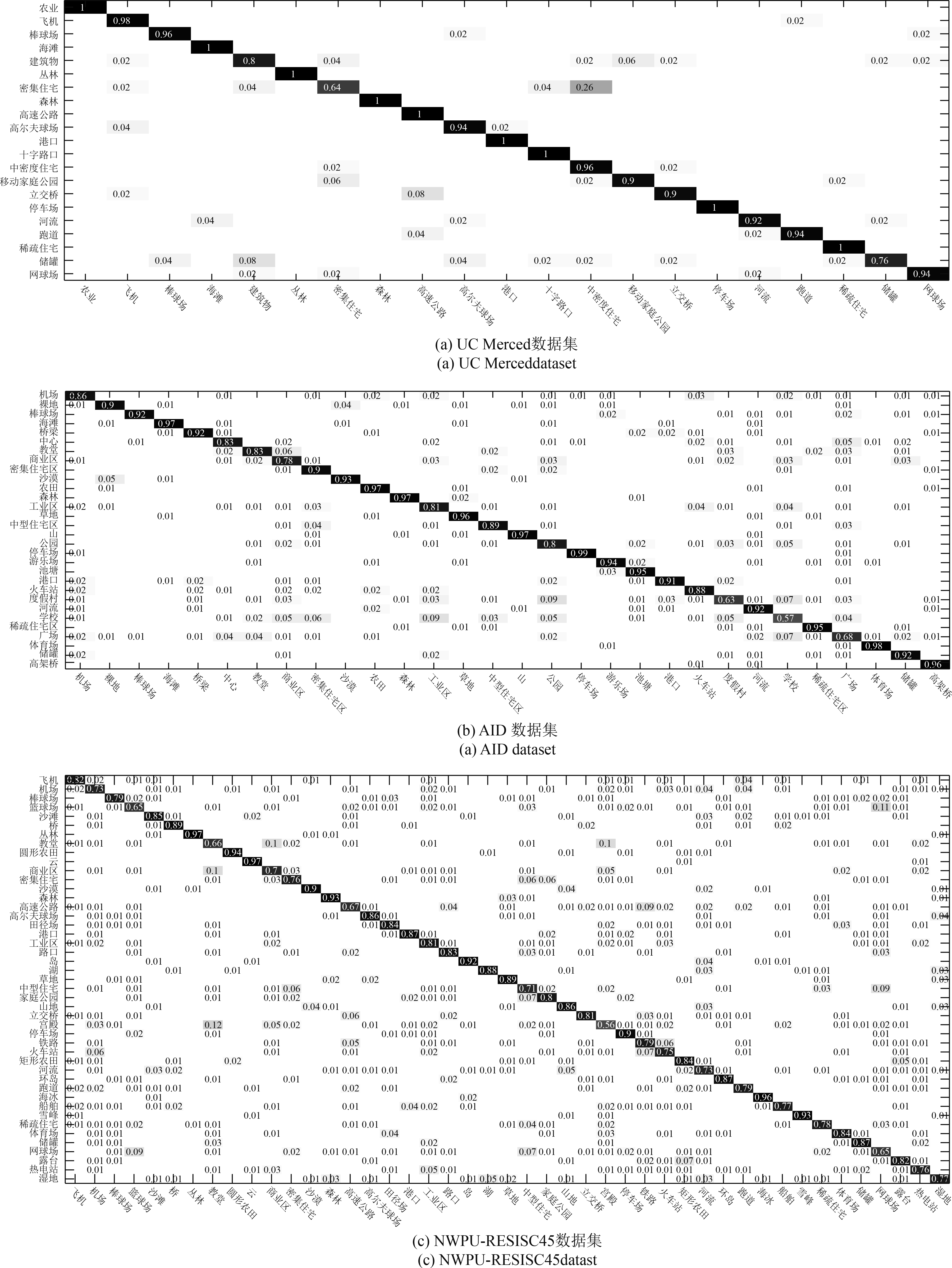
3.4.2 基于混淆矩阵的定量评估
由于篇幅所限,本文只展示了CH(手工特征)、BoVW_CH(基于CH手工特征进行编码)、AlexNet和VGG-16(数据驱动特征)在3个数据集上的混淆矩阵,训练率均为50%,由于篇幅所限,正文部分只展示了BoVW_CH和VGG-16的混淆矩阵,如图4、5所示,CH和AlexNet的混淆矩阵参见电子版附录(DOI:10.11834/jrs.20188015)。本文根据矩阵中数值的大小对其进行了不同程度的标黑,数值越大标黑越明显,显然,矩阵对角线部分越黑,说明混淆程度越低,场景分类表现越好。


从混淆矩阵的对比中可以得到以下结果:
(1) 基于SIFT特征所得分类结果的混淆程度最高,基于CH特征所得分类结果的混淆主要集中在颜色特征比较相近的类别之间,如高尔夫球场和草地两个颜色相近的类别;
(2) 在所有的特征提取策略中,手工特征所得分类结果的混淆程度最高,数据驱动特征所得分类结果的混淆程度最低;
(3) 所有特征提取策略在UC Merced数据集上的混淆程度最低,在AID和NWPU-RESISC45数据集上的混淆程度偏高。
3.4.3 基于Kappa系数的定量评估
不同特征提取策略在UC Merced、AID和NWPU-RESISC45数据集上的Kappa系数如表4所示。
表 4 基于29种特征提取策略的Kappa系数
Table 4 Kappa coefficient of 29 kinds of feature extraction strategies
| 特征 | UC-Merced | AID | NWPU-RESISC45 | ||||||
| (20%) | (50%) | (20%) | (50%) | (20%) | (50%) | ||||
| CH | 0.3500 | 0.3680 | 0.3221 | 0.3503 | 0.3165 | 0.3306 | |||
| LBP | 0.2700 | 0.3280 | 0.2361 | 0.2681 | 0.2041 | 0.2376 | |||
| SIFT | 0.2338 | 0.2540 | 0.1100 | 0.1383 | 0.0927 | 0.1076 | |||
| GIST | 0.3269 | 0.3940 | 0.2764 | 0.3286 | 0.1741 | 0.2062 | |||
| CH | BoVW | 0.5413 | 0.6870 | 0.4610 | 0.5322 | 0.5015 | 0.5418 | ||
| IFK | 0.6294 | 0.7860 | 0.6427 | 0.7260 | 0.6532 | 0.7134 | |||
| LLC | 0.5356 | 0.6240 | 0.4743 | 0.5143 | 0.4634 | 0.4764 | |||
| pLSA | 0.4450 | 0.5330 | 0.4151 | 0.4443 | 0.4076 | 0.4308 | |||
| SPM | 0.4444 | 0.5550 | 0.4004 | 0.4504 | 0.4035 | 0.4459 | |||
| VLAD | 0.5131 | 0.6250 | 0.4246 | 0.5218 | 0.4976 | 0.5758 | |||
| LBP | BoVW | 0.5881 | 0.6960 | 0.5324 | 0.6201 | 0.3997 | 0.4038 | ||
| IFK | 0.6238 | 0.7510 | 0.6453 | 0.7411 | 0.5349 | 0.6140 | |||
| LLC | 0.5188 | 0.6290 | 0.5147 | 0.5387 | 0.3598 | 0.3607 | |||
| pLSA | 0.4938 | 0.6020 | 0.3915 | 0.4356 | 0.3489 | 0.3739 | |||
| SPM | 0.4331 | 0.5490 | 0.3449 | 0.4400 | 0.3414 | 0.3883 | |||
| VLAD | 0.5950 | 0.7240 | 0.5777 | 0.6819 | 0.4528 | 0.5006 | |||
| SIFT | BoVW | 0.6075 | 0.7140 | 0.5928 | 0.6638 | 0.4248 | 0.4416 | ||
| IFK | 0.6594 | 0.7380 | 0.6938 | 0.7723 | 0.5439 | 0.6050 | |||
| LLC | 0.5844 | 0.6800 | 0.5259 | 0.5703 | 0.3690 | 0.3801 | |||
| pLSA | 0.5763 | 0.6640 | 0.4979 | 0.5420 | 0.3883 | 0.4144 | |||
| SPM | 0.4462 | 0.5480 | 0.3411 | 0.4224 | 0.3147 | 0.3816 | |||
| VLAD | 0.5988 | 0.7250 | 0.6342 | 0.7152 | 0.4821 | 0.5403 | |||
| AlexNet | 0.8856 | 0.9290 | 0.8573 | 0.8784 | 0.7854 | 0.8096 | |||
| CaffeNet | 0.8975 | 0.9390 | 0.8641 | 0.8908 | 0.7950 | 0.8239 | |||
| GoogLeNet | 0.8944 | 0.9330 | 0.8274 | 0.8596 | 0.7810 | 0.7962 | |||
| VGG-16 | 0.8981 | 0.9405 | 0.8611 | 0.8981 | 0.8188 | 0.8520 | |||
| VGG-19 | 0.8862 | 0.9290 | 0.8633 | 0.8985 | 0.8122 | 0.8412 | |||
| ResNet-50 | 0.9098 | 0.9536 | 0.8741 | 0.9128 | 0.8393 | 0.8759 | |||
| ResNet-152 | 0.9152 | 0.9667 | 0.8843 | 0.9216 | 0.8487 | 0.8852 | |||
| 注:20%和50%代表训练率,即训练样本数占数据集总样本数的比例。左侧的CH、LBP、SIFT表示不同编码方式所采用的3种底层特征。加粗文字表示Kappa系数值最高的特征提取策略。 | |||||||||
从表4中可以看出:
(1) 手工特征对应的Kappa系数整体偏低,基本都低于0.4;
(2) 手工特征编码在3个数据集上的Kappa系数均处于0.4—0.8,相比手工特征有所提高;
(3) 数据驱动特征所得到的Kappa系数整体较高,均处于0.8—0.95。
3.4.4 基于运算时间和标准差的定量评估
为了评估特征提取策略的效率和稳定性,本文在规模最大的NWPU-RESISC45数据集上计算了所有特征提取策略的运算时间和标准差(训练率为50%),如表5所示,可以看出:
(1) 在手工特征、手工特征编码和数据驱动特征3类特征中,SIFT、SPM和AlexNet的运算时间最少,总体来看,SIFT最少,AlexNet与之相当;
(2) 手工特征编码的运算时间受底层手工特征的影响较大,两者成正比关系;
(3) 在手工特征、手工特征编码和数据驱动特征3类特征中,GIST、IFK_LBP和ResNet-152的标准差最小,总体来看,ResNet-152最小;
(4) 手工特征编码中,基于CH的编码特征所对应的标准差总体小于基于LBP和SIFT的编码特征;
(5) 所有特征提取策略中,数据驱动特征对应的标准差相对较小。
表 5 29种特征提取策略在NWPU-RESISC45上的综合评估
Table 5 Comprehensive evaluation of 29 kinds of feature extraction strategies in terms of NWPU-RESISC45
| 方法 | 总体精度(50%) | 运算时间/s | 标准差(50%) | |
| CH | 34.50±0.29 | 0.1929 | 0.2254 | |
| LBP | 25.24±0.24 | 1.3288 | 0.2290 | |
| SIFT | 12.86±0.36 | 0.0634 | 0.1838 | |
| GIST | 22.22±0.23 | 0.8042 | 0.1598 | |
| CH | BoVW | 54.02±0.34 | 0.2628 | 0.1648 |
| IFK | 72.61±0.30 | 0.2415 | 0.1556 | |
| LLC | 47.96±0.31 | 0.3381 | 0.1974 | |
| pLSA | 44.02±0.48 | 0.2044 | 0.1970 | |
| SPM | 45.49±0.29 | 0.1915 | 0.1962 | |
| VLAD | 58.75±0.33 | 0.2669 | 0.1747 | |
| LBP | BoVW | 40.82±0.29 | 1.4435 | 0.1938 |
| IFK | 62.03±0.30 | 1.4876 | 0.1537 | |
| LLC | 37.17±0.29 | 1.6085 | 0.1988 | |
| pLSA | 38.48±0.23 | 1.3384 | 0.2062 | |
| SPM | 40.81±0.27 | 1.3235 | 0.2020 | |
| VLAD | 51.73±0.32 | 1.4100 | 0.1834 | |
| SIFT | BoVW | 44.34±0.36 | 0.1420 | 0.2031 |
| IFK | 61.10±0.36 | 0.1749 | 0.1773 | |
| LLC | 38.66±0.23 | 0.2078 | 0.1927 | |
| pLSA | 43.02±0.32 | 0.0723 | 0.2001 | |
| SPM | 39.02±0.21 | 0.0591 | 0.2153 | |
| VLAD | 54.78±0.31 | 0.1129 | 0.1902 | |
| AlexNet | 82.17±0.35 | 0.0662 | 0.0992 | |
| CaffeNet | 82.84±0.15 | 0.3703 | 0.0970 | |
| GoogLeNet | 79.87±0.23 | 0.2967 | 0.1196 | |
| VGG-16 | 85.19±0.21 | 0.4344 | 0.0834 | |
| VGG-19 | 84.66±0.22 | 0.4547 | 0.0925 | |
| ResNet-50 | 87.61±0.17 | 0.5946 | 0.0781 | |
| ResNet-152 | 88.53±0.46 | 0.8985 | 0.0702 | |
| 注:50%代表训练率,即训练样本数占数据集总样本数的比例。左侧的CH、LBP、SIFT表示不同编码方式所采用的3种底层特征。 | ||||
3.5 定量评估结果分析
3.5.1 综合分析
如表5所示,本文对29种特征提取策略的总体精度、运算时间和标准差在规模最大的NWPU-RESISC45数据集(训练率为50%)上进行了综合评估,再结合表1—表4、图4和图5中的定量对比数据,可得到以下结论:
综合分类精度、效率和稳定性来看,各类特征提取策略各有特点。数据驱动特征的分类精度和稳定性较好,但是运算效率不占优势(AlexNet除外),而且一般都需要大量的人工标注样本,适用于对分类精度和稳定性要求较高、且计算资源和标注样本比较丰富的场合。
手工特征及手工特征编码的分类精度和稳定性虽不及数据驱动特征,但是运算效率较高(LBP及其编码特征除外),而且算法本身不需要大量的训练样本,适用于对实时性要求较高且人工标注样本数量较少的场合。手工特征的另一项优势在于引入了先验知识,体现了人对地物特征的分析和理解,可将手工特征与数据驱动特征进行深度融合,如用于改进CNN模型架构,改善CNN模型的参数初始化等。
总体来看,在29种特征提取策略中,AlexNet综合性能最佳,它的网络层数相对较少,因此运算速度很快(与最快的SIFT相当),且分类精度和稳定性也相对较高。因此,AlexNet这种网络层数相对较少的深度学习特征适合综合要求较高的场合。
3.5.2 逐类分析
即便使用同一种特征提取策略,各类的分类精度和各类之间的混淆程度也不一样,这与各类场景的地貌特征有很大的关系。因此,本文从地物特点的角度出发,对不同场景类别的分类结果进行了逐类分析。首先,本文采用目前使用较为广泛的VGG-16作为特征提取方法,可得到AID数据库(50%的训练率)上的混淆矩阵,如图5(b)所示,图中对角线的数据表示分类正确的比例,对角线以外的数据表示分类发生混淆的比例。然后,依据该表格的数值对各个场景的分类结果进行了细化分析,结论如下:
(1) 从对角线的数据可以看出,中心区、火车站、度假村和学校等几个场景类别的分类精度远低于总体精度,教堂、商业区、工业区、公园、广场和体育场等几个场景类别的分类精度略低于总体精度;
(2) 从对角线以外的数据可以看出,分类混淆主要发生在中心区、教堂、工业区、学校和商业区等几个场景类别之间,这可能是因为这几类场景中都包含有相似的建筑物结构。其余的类别中,广场、体育场和游乐场之间以及裸地和沙漠之间均存在一定程度的分类混淆,广场、体育场和游乐场这几类场景中均包含有空旷的场所,而裸地和沙漠这两类场景本身的地貌特征就很相似,这些可能是导致这几类场景混淆比例较高的原因。
3.6 高分辨率遥感图像数据集的复杂度对比
本文将所有对比算法在3个数据集上的定量指标按照数据集的不同进行综合对比,对3个数据集的复杂度和挑战性进行定量的对比。如表6所示,给出了所有算法在3个数据库上的总体精度和Kappa系数的均值。
表 6 3个数据集上的总体精度和Kappa系数均值对比
Table 6 Comparison of mean value of overall accuracy and Kappa coefficient on three datasets
| 数据集 | 总体精度 | Kappa系数 | |||
| 20% | 50% | 20% | 50% | ||
| UC-Merced | 62.45 | 69.67 | 0.5966 | 0.6845 | |
| AID | 57.19 | 62.18 | 0.5547 | 0.6095 | |
| NWPU-RESISC45 | 50.38 | 53.81 | 0.4950 | 0.5295 | |
| 注:20%和50%代表训练率,即训练样本数占数据集总样本数的比例。各列数值最低的数据被加粗,代表数据集复杂度最高。 | |||||
通过表6中的数值对比可以看出,UC Merced数据集上的结果最好,AID次之,NWPU-RESISC45最差。由此看出,NWPU-RESISC45数据集的复杂度最高、挑战性最强,经典的UC Merced数据集复杂度最低、挑战性最弱,这与前文的数据库描述(新提出的数据集样本规模较大、场景类别丰富、类间相似性和类内多样性较高)相吻合。近些年,随着深度学习的发展,基于数据驱动特征的场景分类方法已经能够在早期提出的UC Merced等复杂度不高的数据集上取得较高的成绩,此类数据集已经不太适用于检验新方法的性能,最近提出的大规模数据集对特征提取策略更具挑战性。
表 7 基于VGG-16特征的场景分类方法在AID数据集上的混淆矩阵表格
Table 7 Confusion matrix of scene classification based on VGG-16 features on AID dataset
| 预测实际 | 机场 | 裸地 | 棒球场 | 海滩 | 桥梁 | 中心区 | 教堂 | 商业区 | 密集住
宅区 |
沙漠 | 农田 | 森林 | 工业区 | 草地 | 中型住
宅区 |
山 | 公园 | 停车场 | 游乐场 | 池塘 | 港口 | 火车站 | 度假村 | 河流 | 学校 | 稀疏住
宅区 |
广场 | 体育场 | 储罐 | 高架桥 |
| 机场 | 0.89 | 0.01 | 0.01 | 0.01 | 0.01 | 0.03 | 0.01 | 0.01 | 0.01 | 0.01 | 0.01 | 0.01 | 0.01 | 0.01 | ||||||||||||||||
| 裸地 | 0.01 | 0.91 | 0.01 | 0.04 | 0.01 | 0.03 | 0.01 | |||||||||||||||||||||||
| 棒球场 | 0.95 | 0.01 | 0.01 | 0.01 | 0.01 | 0.01 | ||||||||||||||||||||||||
| 海滩 | 0.01 | 0.98 | 0.01 | 0.01 | 0.01 | 0.01 | ||||||||||||||||||||||||
| 桥梁 | 0.01 | 0.91 | 0.01 | 0.01 | 0.01 | 0.01 | 0.01 | 0.01 | 0.02 | 0.01 | 0.01 | |||||||||||||||||||
| 中心区 | 0.01 | 0.02 | 0.7 | 0.04 | 0.02 | 0.04 | 0.01 | 0.02 | 0.01 | 0.04 | 0.08 | 0.03 | 0.02 | 0.01 | ||||||||||||||||
| 教堂 | 0.02 | 0.8 | 0.02 | 0.03 | 0.01 | 0.03 | 0.05 | 0.01 | 0.04 | 0.01 | ||||||||||||||||||||
| 商业区 | 0.01 | 0.85 | 0.01 | 0.02 | 0.03 | 0.01 | 0.01 | 0.01 | 0.06 | |||||||||||||||||||||
| 密集住宅区 | 0.01 | 0.01 | 0.93 | 0.01 | 0.02 | 0.01 | ||||||||||||||||||||||||
| 沙漠 | 0.03 | 0.01 | 0.95 | 0.01 | 0.01 | |||||||||||||||||||||||||
| 农田 | 0.01 | 0.02 | 0.94 | 0.01 | 0.02 | 0.02 | ||||||||||||||||||||||||
| 森林 | 0.01 | 0.98 | 0.01 | 0.01 | ||||||||||||||||||||||||||
| 工业区 | 0.01 | 0.02 | 0.01 | 0.03 | 0.01 | 0.8 | 0.01 | 0.01 | 0.04 | 0.03 | 0.03 | |||||||||||||||||||
| 草地 | 0.01 | 0.01 | 0.01 | 0.98 | ||||||||||||||||||||||||||
| 中型住宅区 | 0.01 | 0.03 | 0.93 | 0.01 | 0.01 | 0.01 | ||||||||||||||||||||||||
| 山 | 0.01 | 0.01 | 0.01 | 0.98 | ||||||||||||||||||||||||||
| 公园 | 0.02 | 0.01 | 0.01 | 0.82 | 0.02 | 0.01 | 0.01 | 0.03 | 0.03 | 0.03 | 0.02 | 0.01 | ||||||||||||||||||
| 停车场 | 0.01 | 0.01 | 0.01 | 0.01 | 0.97 | 0.01 | ||||||||||||||||||||||||
| 游乐场 | 0.01 | 0.02 | 0.95 | 0.01 | 0.02 | 0.01 | 0.01 | |||||||||||||||||||||||
| 池塘 | 0.01 | 0.94 | 0.02 | 0.01 | ||||||||||||||||||||||||||
| 港口 | 0.01 | 0.01 | 0.01 | 0.01 | 0.96 | 0.01 | 0.01 | 0.01 | ||||||||||||||||||||||
| 火车站 | 0.02 | 0.02 | 0.03 | 0.02 | 0.02 | 0.05 | 0.79 | 0.01 | 0.01 | 0.02 | 0.01 | 0.01 | 0.01 | |||||||||||||||||
| 度假村 | 0.01 | 0.01 | 0.01 | 0.01 | 0.04 | 0.02 | 0.04 | 0.05 | 0.69 | 0.01 | 0.06 | 0.01 | 0.01 | 0.01 | 0.01 | |||||||||||||||
| 河流 | 0.01 | 0.01 | 0.02 | 0.92 | ||||||||||||||||||||||||||
| 学校 | 0.03 | 0.01 | 0.01 | 0.06 | 0.01 | 0.07 | 0.01 | 0.01 | 0.01 | 0.01 | 0.04 | 0.7 | 0.01 | |||||||||||||||||
| 稀疏住宅区 | 0.01 | 0.01 | 0.02 | 0.01 | 0.94 | 0.01 | 0.01 | |||||||||||||||||||||||
| 广场 | 0.02 | 0.01 | 0.03 | 0.01 | 0.02 | 0.01 | 0.01 | 0.01 | 0.07 | 0.8 | 0.01 | 0.01 | ||||||||||||||||||
| 体育场 | 0.06 | 0.01 | 0.01 | 0.05 | 0.01 | 0.01 | 0.02 | 0.84 | 0.01 | |||||||||||||||||||||
| 储罐 | 0.01 | 0.01 | 0.01 | 0.01 | 0.01 | 0.01 | 0.01 | 0.01 | 0.03 | 0.01 | 0.01 | 0.01 | 0.89 | 0.01 | ||||||||||||||||
| 高架桥 | 0.01 | 0.98 | ||||||||||||||||||||||||||||
| 注:表中对数据进行加黑处理,加黑的程度与数值大小成正比。 | ||||||||||||||||||||||||||||||
4 结 论
本文对现有高分辨率遥感图像场景分类方法常用的特征提取策略进行了分类总结,从理论分析和实验对比两个层面将特征提取策略对场景分类性能的影响进行了定性和定量评估,并对参与实验评估的3个数据库的复杂度进行了评估,得到以下结论:(1)手工特征的分类精度较低,稳定性较差,但是算法运算效率较高,与其他高层特征组合能够提升综合分类性能;(2)在所有特征提取策略中,手工特征编码在分类精度、效率以及稳定性等方面均处于中等水平;(3)数据驱动特征的分类精度和稳定性相对较好,但是运算效率大部分较低;(4)层数相对较少的深度学习特征AlexNet,综合性能较强,适合对分类精度、算法效率和稳定性均有要求的场合;(5)通过对混淆矩阵的定量分析,发现一些属于土地使用类型的场景因为标志建筑物或场所较为相似而容易发生混淆;一些属于土地覆盖类型的场景因为具有相似的地貌特征而容易发生混淆;(6)根据所有对比算法在3个数据集上的定量指标均值对比,规模最大的NWPU-RESISC45数据集复杂度最高,挑战性最强。
目前,基于CNN特征的分类表现优异,是本领域的研究重点,相比于CNN特征,人工特征的优势在于引入了先验知识,体现了人对地物特征的分析和理解,这些知识可用于CNN模型的优化、缩短训练时间、精简网络层级,甚至是改进整个模型。因此,将手工特征的先验知识引入CNN模型将是未来的发展方向之一。另一方面,CNN的训练存在参数初始化以及需要大量样本的问题:随机初始化网络参数容易让训练收敛到局部极值点,大规模的样本人工标注代价较高。目前常用的解决方法是采用弱监督训练,即:先在大规模的自然场景图像库ImageNet上进行预训练,然后再利用少量的遥感图像样本进行微调。将生成式对抗网络GAN(Generative Adversarial Networks)引入CNN的训练也可能会是下一步的研究热点之一,它的作用体现在:(1)在训练过程中,GAN可以对CNN的参数进行无监督初始化;(2)GAN能够对现有样本进行扩充。
此外,本文主要在公开的数据集上进行实验评估,由于这些数据集的图片是只包含有3个通道的伪彩图像,因此实验中无法利用图像的光谱信息进行分析,在实际应用中,NDVI、NDWI等遥感参量和多谱段信息对场景分类无疑具有重要作用,将NDVI、NDWI等遥感参量、多谱段信息和目前各种特征提取策略进行融合也是下一步研究工作的重点之一。

参考文献(References)
-
Aptoula E. 2014. Remote sensing image retrieval with global morphological texture descriptors. IEEE Transactions on Geoscience and Remote Sensing, 52 (5): 3023–3034. [DOI: 10.1109/TGRS.2013.2268736]
-
Avramović A and Risojević V. 2016. Block-based semantic classification of high-resolution multispectral aerial images. Signal, Image and Video Processing, 10 (1): 75–84. [DOI: 10.1007/s11760-014-0704-x]
-
Bengio Y, Lamblin P, Popovici D and Larochelle H. 2007. Greedy layer-wise training of deep networks//Proceedings of the 20th Annual Conference on Neural Information Processing Systems. Vancouver, British Columbia, Canada: MIT Press: 153–160
-
Bhagavathy S and Manjunath B S. 2006. Modeling and detection of geospatial objects using texture motifs. IEEE Transactions on Geoscience and Remote Sensing, 44 (12): 3706–3715. [DOI: 10.1109/TGRS.2006.881741]
-
Blaschke T. 2003. Object-based contextual image classification built on image segmentation//Proceedings of 2003 IEEE Workshop on Advances in Techniques for Analysis of Remotely Sensed Data. Greenbelt, MD, USA, USA: IEEE: 113–119 [DOI: 10.1109/WARSD.2003.1295182]
-
Blaschke T. 2010. Object based image analysis for remote sensing. ISPRS Journal of Photogrammetry and Remote Sensing, 65 (1): 2–16. [DOI: 10.1016/j.isprsjprs.2009.06.004]
-
Blei D M, Ng A Y and Jordan M I. 2003. Latent dirichlet allocation. Journal of Machine Learning Research, 3 : 993–1022. [DOI: 10.1162/jmlr.2003.3.4-5.993]
-
Bosch A, Zisserman A and Muñoz X. 2006. Scene classification via pLSA//Proceedings of the 9th European Conference on Computer Vision. Graz, Austria: Springer: 517–530 [DOI: 10.1007/11744085_40]
-
Chaib S, Gu Y F and Yao H X. 2016a. An informative feature selection method based on sparse pca for vhr scene classification. IEEE Geoscience and Remote Sensing Letters, 13 (2): 147–151. [DOI: 10.1109/LGRS.2015.2501383]
-
Chaib S, Gu Y F, Yao H X and Zhao S C. 2016b. A VHR scene classification method integrating sparse PCA and saliency computing//Proceedings of 2016 IEEE International Geoscience and Remote Sensing Symposium. Beijing, China: IEEE: 2742–2745 [DOI: 10.1109/IGARSS.2016.7729708]
-
Chen G Y, Li X and Liu L. 2016. A study on the recognition and classification method of high resolution remote sensing image based on deep belief network//Gong M G, Pan L Q, Song T and Zhang G X, eds. Bio-Inspired Computing - Theories and Applications. Singapore: Springer: 362–370 [DOI: 10.1007/978-981-10-3611-8_29]
-
Chen L J, Yang W, Xu K and Xu T. 2011. Evaluation of local features for scene classification using VHR satellite images//Proceedings of 2011 Joint Urban Remote Sensing Event. Munich, Germany: IEEE: 385–388 [DOI: 10.1109/JURSE.2011.5764800]
-
Chen Y S, Zhao X and Jia X P. 2015. Spectral–spatial classification of hyperspectral data based on deep belief network. IEEE Journal of Selected Topics in Applied Earth Observations and Remote Sensing, 8 (6): 2381–2392. [DOI: 10.1109/JSTARS.2015.2388577]
-
Cheng G, Han J W and Lu X Q. 2017a. Remote sensing image scene classification: benchmark and state of the art. Proceedings of the IEEE, 105 (10): 1865–1883. [DOI: 10.1109/JPROC.2017.2675998]
-
Cheng G, Li Z P, Yao X W, Guo L and Wei Z L. 2017b. Remote sensing image scene classification using bag of convolutional features. IEEE Geoscience and Remote Sensing Letters, 14 (10): 1735–1739. [DOI: 10.1109/LGRS.2017.2731997]
-
Cheriyadat A M. 2014. Unsupervised feature learning for aerial scene classification. IEEE Transactions on Geoscience and Remote Sensing, 52 (1): 439–451. [DOI: 10.1109/TGRS.2013.2241444]
-
Comon P. 1994. Independent component analysis, a new concept?. Signal Processing, 36 (3): 287–314. [DOI: 10.1016/0165-1684(94)90029-9]
-
Cousin A, Forni O, Maurice S, Lasue J, Gasnault O and Wiens R. 2011. Independent component analysis classification for chemcam remote sensing data//Proceedings of the 42nd Lunar and Planetary Science Conference. The Woodlands, Texas: [s.n.]
-
Dai D X and Yang W. 2011. Satellite image classification via two-layer sparse coding with biased image representation. IEEE Geoscience and Remote Sensing Letters, 8 (1): 173–176. [DOI: 10.1109/LGRS.2010.2055033]
-
Dell’Acqua F, Gamba P, Ferrari A, Palmason J A, Benediktsson J A and Arnason K. 2004. Exploiting spectral and spatial information in hyperspectral urban data with high resolution. IEEE Geoscience and Remote Sensing Letters, 1 (4): 322–326. [DOI: 10.1109/LGRS.2004.837009]
-
dos Santos J A, Penatti O A B and da Silva Torres R. 2010. Evaluating the potential of texture and color descriptors for remote sensing image retrieval and classification//International Conference on Computer Vision Theory and Applications. Angers, France: [s.n.]: 203–208
-
Du B, Xiong W, Wu J, Zhang L F, Zhang L P and Tao D C. 2017. Stacked convolutional denoising auto-encoders for feature representation. IEEE Transactions on Cybernetics, 47 (4): 1017–1027. [DOI: 10.1109/TCYB.2016.2536638]
-
Du Q, Kopriva I and Szu H H. 2006. Independent-component analysis for hyperspectral remote sensing imagery classification. Optical Engineering, 45 (1): 017008 [DOI: 10.1117/1.2151172]
-
Fan R E, Chang K W, Hsieh C J, Wang X R and Lin C J. 2008. Liblinear: a library for large linear classification. Journal of Machine Learning Research, 9 : 1871–1874. [DOI: 10.1145/1390681.1442794]
-
Gao Y, Mas J F, Maathuis B H P, Zhang X M and Dijk P M V. 2006. Comparison of pixel-based and object-oriented image classification approaches—a case study in a coal fire area, wuda, inner mongolia, China. International Journal of Remote Sensing, 27 (18): 4039–4055. [DOI: 10.1080/01431160600702632]
-
Gong Z Q, Zhong P, Yu Y and Hu W D. 2018. Diversity-promoting deep structural metric learning for remote sensing scene classification. IEEE Transactions on Geoscience and Remote Sensing, 56 (1): 371–390. [DOI: 10.1109/TGRS.2017.2748120]
-
Guo X, Huang X, Zhang L F, Zhang L P, Plaza A and Benediktsson J A. 2016. Support tensor machines for classification of hyperspectral remote sensing imagery. IEEE Transactions on Geoscience and Remote Sensing, 54 (6): 3248–3264. [DOI: 10.1109/TGRS.2016.2514404]
-
Han J W, Zhou P C, Zhang D W, Cheng G, Guo L, Liu Z B, Bu S H and Wu J. 2014. Efficient, simultaneous detection of multi-class geospatial targets based on visual saliency modeling and discriminative learning of sparse coding. ISPRS Journal of Photogrammetry and Remote Sensing, 89 : 37–48. [DOI: 10.1016/j.isprsjprs.2013.12.011]
-
Han W, Feng R Y, Wang L Z and Cheng Y F. 2017. A semi-supervised generative framework with deep learning features for high-resolution remote sensing image scene classification. ISPRS Journal of Photogrammetry and Remote Sensing [DOI: 10.1016/j.isprsjprs.2017.11.004]
-
Haralick R M, Shanmugam K and Dinstein I H. 1973. Textural features for image classification. IEEE Transactions on Systems, Man, and Cybernetics, SMC-3 (6): 610–621. [DOI: 10.1109/TSMC.1973.4309314]
-
He K M, Zhang X Y, Ren S Q and Sun J. 2014. Spatial pyramid pooling in deep convolutional networks for visual recognition. IEEE Transactions on Pattern Analysis and Machine Intelligence, 37 (9): 1904–1916. [DOI: 10.1109/TPAMI.2015.2389824]
-
He K M, Zhang X Y, Ren S Q and Sun J. 2016. Deep residual learning for image recognition//Proceedings of 2016 IEEE Conference on Computer Vision and Pattern Recognition. Las Vegas, NV, USA: IEEE: 770–778 [DOI: 10.1109/CVPR.2016.90]
-
Hinton G E, Osindero S and Teh Y W. 2006. A fast learning algorithm for deep belief nets. Neural Computation, 18 (7): 1527–1554. [DOI: 10.1162/neco.2006.18.7.1527]
-
Hinton G E and Salakhutdinov R R. 2006. Reducing the dimensionality of data with neural networks. Science, 313 (5786): 504–507. [DOI: 10.1126/science.1127647]
-
Hou B, Luo X H, Wang S, Jiao L C and Zhang X R. 2015. Polarimetric SAR images classification using deep belief networks with learning features//Proceedings of 2015 IEEE International Geoscience and Remote Sensing Symposium. Milan, Italy: IEEE: 2366–2369 [DOI: 10.1109/IGARSS.2015.7326284]
-
Hu F, Xia G S, Hu J W and Zhang L P. 2015a. Transferring deep convolutional neural networks for the scene classification of high-resolution remote sensing imagery. Remote Sensing, 7 (11): 14680–14707. [DOI: 10.3390/rs71114680]
-
Hu J W, Jiang T B, Tong X Y, Xia G S and Zhang L P. 2015b. A benchmark for scene classification of high spatial resolution remote sensing imagery//Proceedings of 2015 IEEE International Geoscience and Remote Sensing Symposium. Milan, Italy: IEEE: 5003–5006 [DOI: 10.1109/IGARSS.2015.7326956]
-
Hu J W, Xia G S, Hu F, Sun H and Zhang L P. 2015c. A comparative study of sampling analysis in scene classification of high-resolution remote sensing imagery//Proceedings of 2015 IEEE International Geoscience and Remote Sensing Symposium. Milan, Italy: IEEE: 14988–15013 [DOI: 10.1109/IGARSS.2015.7326290]
-
Jégou H, Perronnin F, Douze M, Sánchez J, Pérez P and Schmid C. 2012. Aggregating local image descriptors into compact codes. IEEE Transactions on Pattern Analysis and Machine Intelligence, 34 (9): 1704–1716. [DOI: 10.1109/TPAMI.2011.235]
-
Jain A K, Ratha N K and Lakshmanan S. 1997. Object detection using gabor filters. Pattern Recognition, 30 (2): 295–309. [DOI: 10.1016/S0031-3203(96)00068-4]
-
Jia Y Q, Shelhamer E, Donahue J, Karayev S, Long J, Girshick R, Guadarrama S and Darrell T. 2014. Caffe: convolutional architecture for fast feature embedding//Proceedings of the 22nd ACM International Conference on Multimedia. Orlando, Florida, USA: ACM: 675–678 [DOI: 10.1145/2647868.2654889]
-
Jolliffe I T. 2005. Pincipal component analysis. Journal of Marketing Research, 87 (100): 513 [DOI: 10.1002/0470013192.bsa501]
-
Karoui M S, Deville Y, Hosseini S, Ouamri A and Ducrot D. 2009. Improvement of remote sensing multispectral image classification by using independent component analysis//Proceedings of the 1st Workshop on Hyperspectral Image and Signal Processing: Evolution in Remote Sensing. Grenoble, France: IEEE: 1–4 [DOI: 10.1109/WHISPERS.2009.5289033]
-
Kasapoglu N G and Ersoy O K. 2007. Border vector detection and adaptation for classification of multispectral and hyperspectral remote sensing images. IEEE Transactions on Geoscience and Remote Sensing, 45 (12): 3880–3893. [DOI: 10.1109/TGRS.2007.900699]
-
Krizhevsky A, Sutskever I and Hinton G E. 2012. Imagenet classification with deep convolutional neural networks// Proceedings of the 25th International Conference on Neural Information Processing Systems. Lake Tahoe, Nevada: ACM: 1097–1105
-
Lazebnik S, Schmid C and Ponce J. 2006. Beyond bags of features: spatial pyramid matching for recognizing natural scene categories//Proceedings of 2006 IEEE Computer Society Conference on Computer Vision and Pattern Recognition. New York, NY, USA: IEEE: 2169–2178 [DOI: 10.1109/CVPR.2006.68]
-
Li F F and Perona P. 2005. A Bayesian hierarchical model for learning natural scene categories//Proceedings of 2005 IEEE Computer Society Conference on Computer Vision and Pattern Recognition. San Diego, CA, USA: IEEE: 524–531 [DOI: 10.1109/CVPR.2005.16]
-
Li H T, Gu H Y, Han Y S and Yang J H. 2010. Object-oriented classification of high-resolution remote sensing imagery based on an improved colour structure code and a support vector machine. International Journal of Remote Sensing, 31 (6): 1453–1470. [DOI: 10.1080/01431160903475266]
-
Liu Q S, Hang R L, Song H H and Li Z. 2018. Learning multiscale deep features for high-resolution satellite image scene classification. IEEE Transactions on Geoscience and Remote Sensing, 56 (1): 117–126. [DOI: 10.1109/TGRS.2017.2743243]
-
Liu Y L, Zhang Y M, Zhang X Y and Liu C L. 2016. Adaptive spatial pooling for image classification. Pattern Recognition, 55 (C): 58–67. [DOI: 10.1016/j.patcog.2016.01.030]
-
Lowe D G. 2004. Distinctive image features from scale-invariant keypoints. International Journal of Computer Vision, 60 (2): 91–110. [DOI: 10.1023/B:VISI.0000029664.99615.94]
-
Luo B, Jiang S J and Zhang L P. 2013. Indexing of remote sensing images with different resolutions by multiple features. IEEE Journal of Selected Topics in Applied Earth Observations and Remote Sensing, 6 (4): 1899–1912. [DOI: 10.1109/JSTARS.2012.2228254]
-
Luus F P S, Salmon B P, van den Bergh F and Maharaj B T J. 2015. Multiview deep learning for land-use classification. IEEE Geoscience and Remote Sensing Letters, 12 (12): 2448–2452. [DOI: 10.1109/LGRS.2015.2483680]
-
Mekhalfi M L, Melgani F, Bazi Y and Alajlan N. 2015. Land-use classification with compressive sensing multifeature fusion. IEEE Geoscience and Remote Sensing Letters, 12 (10): 2155–2159. [DOI: 10.1109/LGRS.2015.2453130]
-
Negrel R, Picard D and Gosselin P H. 2014. Evaluation of second-order visual features for land-use classification//Proceedings of the 12th International Workshop on Content-Based Multimedia Indexing. Klagenfurt, Austria: IEEE: 1–5 [DOI: 10.1109/CBMI.2014.6849835]
-
Newsam S, Wang L, Bhagavathy S and Manjunath B S. 2004. Using texture to analyze and manage large collections of remote sensed image and video data. Applied Optics, 43 (2): 210–217. [DOI: 10.1364/AO.43.000210]
-
Ojala T, Pietikäinen M and Harwood I. 1996. A comparative study of texture measures with classification based on featured distributions. Pattern Recognition, 29 (1): 51–59. [DOI: 10.1016/0031-3203(95)00067-4]
-
Ojala T, Pietikäinen M and Mäenpää T. 2002. Multiresolution gray-scale and rotation invariant texture classification with local binary patterns. IEEE Transactions on Pattern Analysis and Machine Intelligence, 24 (7): 971–987. [DOI: 10.1109/TPAMI.2002.1017623]
-
Oliva A and Torralba A. 2001. Modeling the shape of the scene: a holistic representation of the spatial envelope. International Journal of Computer Vision, 42 (3): 145–175. [DOI: 10.1023/A:1011139631724]
-
Olshausen B A and Field D J. 1997. Sparse coding with an overcomplete basis set: a strategy employed by V1? Vision Research, 37(23): 3311–3325 [DOI: 10.1016/S0042-6989(97)00169-7]
-
Penatti O A B, Nogueira K and dos Santos J A. 2015. Do deep features generalize from everyday objects to remote sensing and aerial scenes domains?//Proceedings of 2015 IEEE Conference on Computer Vision and Pattern Recognition Workshops. Boston, MA, USA: IEEE: 44–51 [DOI: 10.1109/CVPRW.2015.7301382]
-
Perronnin F, Sánchez J and Mensink T. 2010. Improving the fisher kernel for large-scale image classification//Proceedings of the 11th European Conference on Computer Vision. Crete, Greece: Springer: 143–156 [DOI: 10.1007/978-3-642-15561-1_11]
-
Qi K L. 2017. Multi-task classification of high resolution optic remote sensing images based on visual features. Acta Geodaeticaet Cartographica Sinica, 46 (6): 802 [DOI: 10.11947/j.AGCS.2017.20170081] ( 祁昆仑. 2017. 基于视觉特征的高分辨率光学遥感影像多任务分类研究. 测绘学报, 46 (6): 802 [DOI: 10.11947/j.AGCS.2017.20170081] )
-
Risojević V, Momić S and Babić Z. 2011. Gabor descriptors for aerial image classification//Proceedings of the 10th International Conference on Adaptive and Natural Computing Algorithms. Ljubljana, Slovenia: Springer: 51–60 [DOI: 10.1007/978-3-642-20267-4_6]
-
Sermanet P, Eigen D, Zhang X, Mathieu M, Fergus R and LeCun Y. 2014. Overfeat: integrated recognition, localization and detection using convolutional networks. arXiv preprint arXiv:1312.6229
-
Sheng G F, Yang W, Xu T and Sun H. 2012. High-resolution satellite scene classification using a sparse coding based multiple feature combination. International Journal of Remote Sensing, 33 (8): 2395–2412. [DOI: 10.1080/01431161.2011.608740]
-
Shyu C R, Klaric M, Scott G J, Barb A S, Davis C H and Palaniappan K. 2007. Geoiris: geospatial information retrieval and indexing system—content mining, semantics modeling, and complex queries. IEEE Transactions on Geoscience and Remote Sensing, 45 (4): 839–852. [DOI: 10.1109/TGRS.2006.890579]
-
Simonyan K and Zisserman A. 2014. Very deep convolutional networks for large-scale image recognition. arXiv preprint arXiv:1409.1556
-
Sridharan H and Cheriyadat A. 2015. Bag of lines (bol) for improved aerial scene representation. IEEE Geoscience and Remote Sensing Letters, 12 (3): 676–680. [DOI: 10.1109/LGRS.2014.2357392]
-
Swain M J and Ballard D H. 1991. Color indexing. International Journal of Computer Vision, 7 (1): 11–32. [DOI: 10.1007/BF00130487]
-
Szegedy C, Liu W, Jia Y Q, Sermanet P, Reed S, Anguelov D, Erhan D, Vanhoucke V and Rabinovich A. 2015. Going deeper with convolutions//Proceedings of 2015 IEEE Conference on Computer Vision and Pattern Recognition. Boston, MA, USA: IEEE: 1–9 [DOI: 10.1109/CVPR.2015.7298594]
-
Tuia D, Ratle F, Pacifici F, Kanevski M F and Emery W J. 2009. Active learning methods for remote sensing image classification. IEEE Transactions on Geoscience and Remote Sensing, 47 (7): 2218–2232. [DOI: 10.1109/TGRS.2008.2010404]
-
Tuia D, Volpi M, Copa L, Kanevski M and Munoz-Mari J. 2011. A survey of active learning algorithms for supervised remote sensing image classification. IEEE Journal of Selected Topics in Signal Processing, 5 (3): 606–617. [DOI: 10.1109/JSTSP.2011.2139193]
-
Vincent P, Larochelle H, Lajoie I, Bengio Y and Manzagol P A. 2010. Stacked denoising autoencoders: learning useful representations in a deep network with a local denoising criterion. Journal of Machine Learning Research, 11 : 3371–3408.
-
Wan L J, Tang K, Li M Z, Zhong Y F and Qin A K. 2015. Collaborative active and semisupervised learning for hyperspectral remote sensing image classification. IEEE Transactions on Geoscience and Remote Sensing, 53 (5): 2384–2396. [DOI: 10.1109/TGRS.2014.2359933]
-
Wang J, Luo C, Huang H Q, Zhao H Z and Wang S Q. 2017a. Transferring pre-trained deep cnns for remote scene classification with general features learned from linear pca network. Remote Sensing, 9 (3): 225 [DOI: 10.3390/rs9030225]
-
Wang J J, Yang J C, Yu K, Lv F J, Huang T and Gong Y H. 2010. Locality-constrained linear coding for image classification//Proceedings of 2010 IEEE Conference on Computer Vision and Pattern Recognition. San Francisco, CA, USA: IEEE: 3360–3367 [DOI: 10.1109/CVPR.2010.5540018]
-
Wang Y B, Zhang L Q, Deng H, Lu J W, Huang H Y, Zhang L, Liu J, Tang H and Xing X Y. 2017b. Learning a discriminative distance metric with label consistency for scene classification. IEEE Transactions on Geoscience and Remote Sensing, 55 (8): 4427–4440. [DOI: 10.1109/TGRS.2017.2692280]
-
Xia G S, Hu J W, Hu F, Shi B G, Bai X, Zhong Y F, Zhang L P and Lu X Q. 2017. Aid: a benchmark data set for performance evaluation of aerial scene classification. IEEE Transactions on Geoscience and Remote Sensing, 55 (7): 3965–3981. [DOI: 10.1109/TGRS.2017.2685945]
-
Xu S H, Mu X D, Zhao P and Ma J. 2016. Scene classification of remote sensing image based on multi-scale feature and deep neural network. Acta Geodaeticaet Cartographica Sinica, 45 (7): 834–840. [DOI: 10.11947/j.AGCS.2016.20150623] ( 许夙晖, 慕晓冬, 赵鹏, 马骥. 2016. 利用多尺度特征与深度网络对遥感影像进行场景分类. 测绘学报, 45 (7): 834–840. [DOI: 10.11947/j.AGCS.2016.20150623] )
-
Xue Z H, Du P J, Li J and Su H J. 2017. Sparse graph regularization for hyperspectral remote sensing image classification. IEEE Transactions on Geoscience and Remote Sensing, 55 (4): 2351–2366. [DOI: 10.1109/TGRS.2016.2641985]
-
Yang J C, Yu K, Gong Y H and Huang T. 2009. Linear spatial pyramid matching using sparse coding for image classification//Proceedings of IEEE Conference on Computer Vision and Pattern Recognition. Miami, FL, USA: IEEE: 1794–1801 [DOI: 10.1109/CVPR.2009.5206757]
-
Yang Y and Newsam S. 2008. Comparing sift descriptors and gabor texture features for classification of remote sensed imagery//Proceedings of the 15th IEEE International Conference on Image Processing. San Diego, CA, USA: IEEE: 1852–1855 [DOI: 10.1109/ICIP.2008.4712139]
-
Yang Y and Newsam S. 2010. Bag-of-visual-words and spatial extensions for land-use classification//Proceedings of the 18th SIGSPATIAL International Conference on Advances in Geographic Information Systems. New York, NY, USA: ACM: 270–279 [DOI: 10.1145/1869790.1869829]
-
Yao X W, Han J W, Cheng G, Qian X M and Guo L. 2016. Semantic annotation of high-resolution satellite images via weakly supervised learning. IEEE Transactions on Geoscience and Remote Sensing, 54 (6): 3660–3671. [DOI: 10.1109/TGRS.2016.2523563]
-
Zhang F, Du B and Zhang L P. 2016. Scene classification via a gradient boosting random convolutional network framework. IEEE Transactions on Geoscience and Remote Sensing, 54 (3): 1793–1802. [DOI: 10.1109/TGRS.2015.2488681]
-
Zhang L F, Zhang L P, Tao D C and Huang X. 2012. On combining multiple features for hyperspectral remote sensing image classification. IEEE Transactions on Geoscience and Remote Sensing, 50 (3): 879–893. [DOI: 10.1109/TGRS.2011.2162339]
-
Zhao B, Zhong Y F, Xia G S and Zhang L P. 2016a. Dirichlet-derived multiple topic scene classification model for high spatial resolution remote sensing imagery. IEEE Transactions on Geoscience and Remote Sensing, 54 (4): 2108–2123. [DOI: 10.1109/TGRS.2015.2496185]
-
Zhao B, Zhong Y F and Zhang L P. 2016b. A spectral–structural bag-of-features scene classifier for very high spatial resolution remote sensing imagery. ISPRS Journal of Photogrammetry and Remote Sensing, 116 : 73–85. [DOI: 10.1016/j.isprsjprs.2016.03.004]
-
Zhao B, Zhong Y F, Zhang L P and Huang B. 2016c. The fisher kernel coding framework for high spatial resolution scene classification. Remote Sensing, 8 (2): 157 [DOI: 10.3390/rs8020157]
-
Zhao L J, Tang P and Huo L Z. 2014. A 2-D wavelet decomposition-based bag-of-visual-words model for land-use scene classification. International Journal of Remote Sensing, 35 (6): 2296–2310. [DOI: 10.1080/01431161.2014.890762]
-
Zhao L L, Tang P and Huo L Z. 2016d. Feature significance-based multibag-of-visual-words model for remote sensing image scene classification. Journal of Applied Remote Sensing, 10 (3): 035004 [DOI: 10.1117/1.JRS.10.035004]
-
Zhao W Z and Du S H. 2016. Scene classification using multi-scale deeply described visual words. International Journal of Remote Sensing, 37 (17): 4119–4131. [DOI: 10.1080/01431161.2016.1207266]
-
Zheng X W, Sun X, Fu K and Wang H Q. 2013. Automatic annotation of satellite images via multifeature joint sparse coding with spatial relation constraint. IEEE Geoscience and Remote Sensing Letters, 10 (4): 652–656. [DOI: 10.1109/LGRS.2012.2216499]
-
Zhong P, Gong Z P, Li S T and Schönlieb C B. 2017. Learning to diversify deep belief networks for hyperspectral image classification. IEEE Transactions on Geoscience and Remote Sensing, 55 (6): 3516–3530. [DOI: 10.1109/TGRS.2017.2675902]
-
Zhong P, Gong Z Q and Schönlieb C. 2016. A diversified deep belief network for hyperspectral image classification. ISPRS-International Archives of the Photogrammetry, Remote Sensing and Spatial Information Sciences, XLI-B7: 443–449 [DOI: 10.5194/isprs-archives-XLI-B7-443-2016]
-
Zhong Y F. 2016. Large patch convolutional neural networks for the scene classification of high spatial resolution imagery. Journal of Applied Remote Sensing, 10 (2): 025006 [DOI: 10.1117/1.JRS.10.025006]
-
Zhu Q Q, Zhong Y F, Zhang L P and Li D R. 2017. Scene classification based on the fully sparse semantic topic model. IEEE Transactions on Geoscience and Remote Sensing, 55 (10): 5525–5538. [DOI: 10.1109/TGRS.2017.2709802]
-
Zou Q, Ni L H, Zhang T and Wang Q. 2015. Deep learning based feature selection for remote sensing scene classification. IEEE Geoscience and Remote Sensing Letters, 12 (11): 2321–2325. [DOI: 10.1109/LGRS.2015.2475299]