
|
收稿日期: 2017-09-14
基金项目: 国家公益气象行业专项(编号:GYHY201406035); 国家青年自然科学基金(编号:41301461)
第一作者简介: 王圆圆(1981— ),女,副研究员,研究方向为生态环境遥感应用。E-mail: wangyuany@cma.gov.cn
中图分类号: P467
文献标识码: A
|
摘要
三峡区域气温变化长期以来受到科研人员和公众的关注。受三峡复杂地形的影响,仅仅基于气象站点观测数据很难准确获取区域气温变化的空间格局,遥感技术则可以通过提供空间连续的地表观测数据来辅助气温变化分析。以广义加性模型GAM(General Additive Model)为插值算法,以高程和夜间地表温度(LSTnight)遥感产品为辅助变量,估算三峡库区1979年—2014年1 km空间分辨率的月气温数据,在此基础上分析了气温变化趋势的时空特征及其与高程和森林覆盖率的关系。研究表明,(1)在插值算法中引入遥感产品LSTnight作为辅助变量可以明显改善气温估算精度,冬春季的改善幅度高于夏秋季;(2)三峡库区年平均气温在1997年后明显上升,但在2003年库区蓄水后无明显变化趋势,几乎所有月(除12月以外)的气温都呈现上升趋势,增温趋势最显著是3月和9月,3月增温主要来自于库区东部山区的贡献,而9月增温主要来自于库区西部平原的贡献;(3)多数月份(除7月、8月、9月以外)的低温上升速度超过高温上升速度,导致区域气温的动态变化范围缩小;(4)三峡库区年平均气温上升速度与高程呈正相关,即海拔越高,升温越快,但在同一海拔高度处,森林覆盖率越高,年均气温上升速度越慢,暗示森林具有抑制增温的作用。
关键词
三峡库区, 气温变化, 广义加性模型, 地表温度
Abstract
The near-surface air temperature (Ta) change in the Three Gorges Dam region (TGD) has long been a popular topic in public and research fields. However, fully capturing the spatial pattern of Ta change in TGD is challenging because of the sparse observation net and complicated topographic conditions. Thermal remote sensing technology can obtain spatially contiguous observations of Land Surface Temperature (LST) in a synoptic manner, thus providing invaluable information for spatial pattern analyses of Ta change given the fact that LST and Ta are closely related. This study aims to obtain the monthly Ta from 1979-2014 and determine its trend at a spatial resolution of 1 km. We used the satellite product of LST at nighttime (LSTnight) as a covariate in the general additive model (GAM), which incorporates spline interpolation and linear regression, to ensure high quality of Ta data. First, monthly Ta estimation accuracies estimated with and without LSTnight were compared to evaluate the contribution of LSTnight. Second, the pixel-wise Ta trend was calculated with the Mann-Kendall method, and the spatial-temporal features of the Ta trend were analyzed. Finally, the effects of elevation and tree cover on the Ta trend were assessed. The main results were as follows. (1) When LSTnight was used as a covariate in GAM, temperature interpolation accuracy dramatically improved. The improvement in the cold season was more obvious than that in the warm season because Ta in the cold season is mainly influenced by LST through a strong radiative cooling effect. (2) Inter-annual variation analysis of regional mean annual Ta in TGD revealed that pronounced warming occurred after 1997, and no significant change in Ta was observed after the water level rose to 135 m in 2003. (3) Temporal-spatial analysis of monthly Ta showed that warming occurs in almost every month (except for December), and the most dramatic warming occurs in March and September. In March, pixels with significant warming trends are mainly located in the eastern mountainous TGD, whereas in September, they are mainly located in the western TGD with a relatively flat terrain. (4) The Ta range for most months has been decreasing because the minimum temperature increased at a faster speed than the maximum temperature. Consequently, the lapse rate of Ta showed a decrease. (5) The enhanced warming trend over high elevations indicated a strong positive correlation between the trend of annual Ta and elevation (r = 0.76). However, when the elevations are similar, the warming trend is less pronounced in regions with dense tree cover, suggesting that forests can restrain warming. We conclude that LSTnight information is beneficial to Ta estimation and that the change trend of Ta in TGD shows various features depending on season, region, land cover properties, and temperature metric. Further in-depth analysis of the driving factors of the Ta trend, such as land use/cover or forest cover change, should be implemented in the future to be fully prepared to meet the challenges of climate change in TGD.
Key words
Three Gorges Dam region (TGD), warming, general additive model, land surface temperature
1 引 言
三峡河谷位于鄂西和渝东的崇山峻岭之中,水流湍急,地形陡峭,气候复杂,兼有山地气候和水域气候特征(于强 等,1996;张强 等,2005;张天宇 等,2010)。在全球变暖的大背景下,世界最大的水电工程—三峡水库的修建对局地气候有何影响,是人们极为关注的议题。对此,前人已做过不少研究(Wu 等,2006;Miller等,2005;陈鲜艳 等,2009;马占山 等,2010;Wu 等,2012;周英和袁久坤,2016),主流意见认为,由于原本植被密集的陡峭山坡变成了平坦水面,气温变化体现在水体对气温的调节作用上,即冬季增温、夏季降温。然而这些研究多数基于站点的分析,虽然数据精度较高、时间序列较长,但缺乏足够的空间代表性。考虑到三峡地区地形复杂、景观破碎度高(Zhao和Shepherd,2012;王圆圆 等,2017),为全面了解区域的气温变化特征,获取高空间分辨率的气温数据非常关键。
在由离散站点气温数据推算空间连续气温时,空间插值是最常用的方法。常用的插值方法一般以高程为辅助变量,可以直接利用经纬度、高程进行3维插值,也可以首先将气温订正到海平面高度,采用基于经纬度的2维插值方法,最后再利用区域DEM和气温直减率获取气温空间分布(李新 等,2003)。插值精度受插值算法的影响,但精度提高潜力很大程度上受制于站网对区域气温空间分布特征的刻画能力(Tietäväinen 等,2010)。出于管理、可进入性等方面的考虑,站点一般布设在海拔较低、地形平坦、人口较密的区域,而这不利于全面捕捉区域气候变化信息。
将卫星遥感数据引入到气温插值中来,是近期一个研究热点(Mostovoy 等,2006;Vancutsem 等,2010;Park,2011;Benali 等,2012;Oyler 等,2015, 2016)。卫星地表温度LST(Land Surface Temperature)与气温紧密相关,虽然就瞬时值而言,两者的关系会受到天气、云量、地表覆盖、辐射、湿度、风速、卫星观测角度等诸多因素的影响(Mostovoy 等,2006;Hill,2013),但就平均值而言,多年平均LST和气温在空间格局上具有非常好的一致性,尤其是不受太阳辐射影响的夜间LST,不仅在格局上与气温接近,在数值上与最低气温也非常接近,可以作为最低气温的替代数据而不会产生很大误差(Mostovoy 等,2006;Vancutsem 等,2010;Oyler 等,2016)。在气温插值中引入LST,可使插值结果继承LST数据中蕴含的丰富空间细节,这些细节体现了受地形特征、土地覆盖等因素影响而造成的近地面能量平衡的变化,是无法从经纬度或高程数据中直接获取的(Oyler 等,2015)。
本文的研究目的是以高程和夜间地表温度(LSTnight)为辅助变量(Wan 等,2004),利用广义加性模型GAM(General Additive Model)算法(Wood,2003),获取三峡库区1979年—2014年1 km空间分辨率的月气温数据,在此基础上,开展气温变化Mann-Kendall斜率(Hamed,2008)的时空格局分析。本文主要侧重分析气温变化趋势的时空特征,不探讨三峡工程的影响,因为这需要考虑更大的空间范围、更多的气象要素,以及相关机理方面的模拟和解释。
2 研究区域、数据和方法
2.2 数据和预处理
2.2.1 地表温度数据(LST)
本文利用了研究区2000年—2014年MOD11A2/LST产品,该产品为8天合成,空间分辨率为1 km,由于夜间LST时空变异性小,与气温关系稳定,因此被选作为GAM气温插值时的辅助信息。遥感数据时间序列短,且受云遮挡的影响,可能有较多缺值,所以我们计算了2000年—2014年每月多年平均LSTnight,以其作为相应月份气温插值时的辅助数据,为保证数据质量,计算时只利用质量标识码为0(即质量最高)的数据。

2.2.2 气象数据
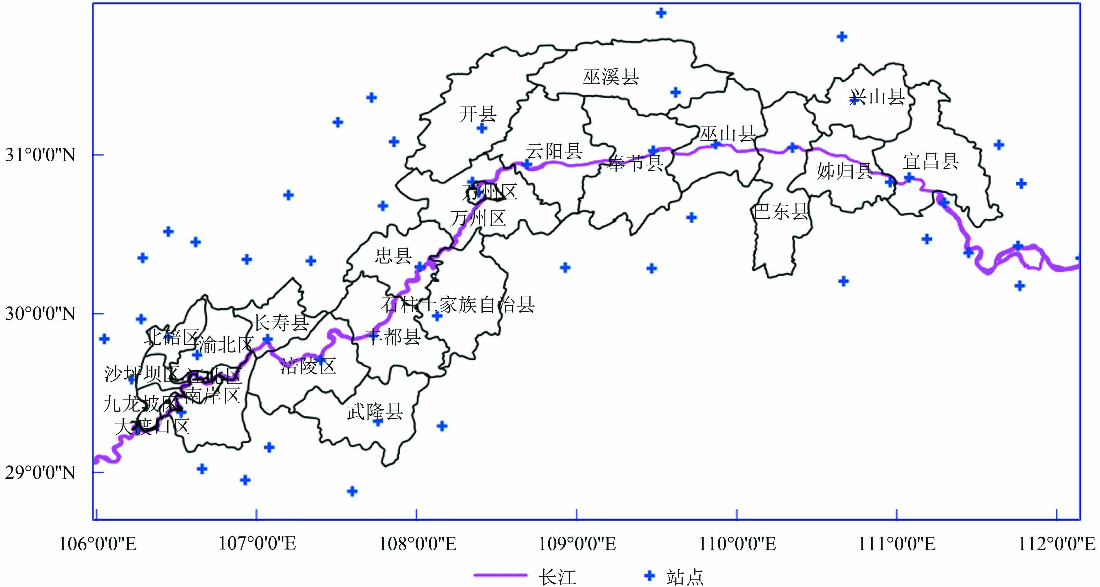
从中国气象数据共享网站上,下载了研究区及附近地区52个站点的1979年—2014年月均气温数据(站点位置如图1),该数据基于“中国国家级地面气象站基本气象要素日值数据集(V3.0)”生成,日值数据经过了严格的质量控制,利用多种检验条件(如气候界限值、台站极值、时间一致性、空间一致性),识别可能有疑误的数据,而后进行人工核查和必要的纠正(任芝花和熊安元,2007)。
2.2.3 数据预处理
根据站点的经纬度,确定其在遥感图像上的位置,为减少定位误差,提取了以站点位置为中心3×3窗口内的平均LSTnight,将站点每年每月的气温数据与该月多年平均的LSTnight进行一一对应。
需要说明的是,受遥感数据时间序列的限制,LSTnight是2000年—2014年的多年月均值,气温数据是1979年—2014年,两者时间跨度虽然不完全一致,但对结果影响不会很大。因为插值时主要利用的是LSTnight描述的地表温度空间格局信息,这种信息在空间上主要受地表覆盖和地形的影响,在时间上主要与季节有关,年际间变化比较小,因此基于2000年—2014年数据统计的每月地表温度格局特征对1979年—2000年也同样适用。不可否认,在30多年的时间跨度上,某些局部地区的地表覆盖会发生变化,但这不会明显改变LSTnight的整体空间格局。
2.3 广义加性模型(GAM)方法介绍
广义加性模型(GAM)具有良好的灵活性、非线性以及对空间数据的平滑处理能力,正日益受到学者关注,前人已开展多项研究,如基于遥感数据估算气温(Parmentier 等,2014)、估算辐射(Ouarda 等,2016;Zhang 等,2016)、评估滑坡可能性(Park和Chi,2008),研究结果表明GAM精度高、过学习风险小,是值得推广应用的方法。
本文采用的GAM模型形式为
| $y = s\left( {\rm {lat,lon}} \right) + b \cdot {\rm {dem}} + c \cdot {\rm {LST}}_{\rm {night}} + d$ | (1) |
式中,y为站点月均温观测值(单位:℃),lat和lon分别为站点纬度和经度,s(lat, lon)表示利用薄盘样条函数对局部做平滑,dem和LSTnight分别为站点的高程(单位:m)和多年平均每月夜间LST(单位:℃),由于LSTnight和高程与气温一般具有线性相关关系,故在GAM模型中作为一个线性的输入。模型(1)中需要估算的参数是s函数的形式(具体为k个局部样条函数的叠加,k为自由度,大小不超过站点个数),dem的斜率b、LSTnight的斜率c、截距d,估算方法是通过最小化目标函数(2)实现
| ${\left\| {y - s} \right\|^2} + {\textit{λ}}\mathop \smallint \nolimits {\left[ {s''} \right]^2}{ \rm {d}}x$ | (2) |
目标函数由模型误差和模型复杂度两部分组成,λ为光滑参数,在误差和复杂度之间起平衡作用,模型参数可以用广义交叉验证GCV(Generalized Cross Validation)或AIC(Akaike’s Information Criterion)为标准进行确定。本文采用了Wood 2003设计了薄盘样条回归函数法,并采用GCV方法确定模型参数,模型代码由R提供(Package ‘mgcv’)。利用每年每月站点的气温数据和辅助信息(即经纬度、DEM、LSTnight)则可以拟合得到一个GAM模型,而后将区域的辅助信息(即经纬度、DEM、LSTnight)输入模型中,则可以得到区域在该年该月的气温插值结果。
3 结果分析
3.1 LSTnight对GAM插值效果的改善
表1显示了两种GAM模型(仅利用高程作为辅助变量,利用高程和LSTnight作为辅助变量)插值均方根误差RMSE(Root Mean Squared Error)的多年月均值,可以看出:(1)GAM气温插值精度很高,RMSE一般在0.39—0.47℃,并具有一定的季节变化:夏季误差偏高,春秋季误差偏低;(2)加入了LSTnight信息后,各月的插值误差都出现明显下降,下降幅度最大(RMSE减少比例超过8%)的是1月—4月以及11月—12月。
表 1 两种GAM模型均方根误差的多年月均值及加入LSTnight后误差减少的比例
Table 1 Monthly temperature interpolation RMSE of two GAM models and the reduction in RMSE when LSTnight was included as a covariate in GAM model
| 月份 | 以DEM作为辅
助变量时的 RMSE/℃ |
以DEM和LSTnight 作为辅助变量 时RMSE/℃ |
加入LSTnight后插
值误差RMSE的 下降幅度/% |
| 1 | 0.46 | 0.41 | –10.71 |
| 2 | 0.45 | 0.40 | –10.40 |
| 3 | 0.45 | 0.41 | –8.88 |
| 4 | 0.43 | 0.39 | –8.50 |
| 5 | 0.42 | 0.40 | –5.16 |
| 6 | 0.41 | 0.39 | –5.78 |
| 7 | 0.46 | 0.44 | –5.12 |
| 8 | 0.46 | 0.43 | –6.35 |
| 9 | 0.44 | 0.41 | –7.01 |
| 10 | 0.42 | 0.40 | –4.38 |
| 11 | 0.44 | 0.40 | –10.55 |
| 12 | 0.47 | 0.41 | –12.04 |
上述结果表明,引入LSTnight信息后,对冬春季气温估算精度的提高幅度高于夏秋季,其他研究也发现类似现象(Oyler 等,2015, 2016),这是因为在冬春季,地表辐射降温作用强,容易造成逆温,气温和高程的关系不明确;而在夏秋季或季风期,气温与高程的相关性强,仅利用高程就可以获取比较高的插值精度。
由GAM获取的三峡库区多年平均气温分布如图3,从图3可以看到明显的地形特征,海拔高处气温低,年均气温小于10℃,河谷以及西部平坦地区气温高,年均气温高于16℃。

3.2 三峡库区区域平均气温的变化趋势
三峡库区年平均气温的时间序列如图4。1979年—2014年,年均气温上升显著,MK斜率为0.23 ℃/10 a(p<1%)。气温的显著增加起始于90年代,到1997年后上升更为明显,气温最高的3个年份为:1998年,2006年,2013年,在这3年中,年均气温都超过了15.7 ℃。如果将时间分为两段:1979年—1997年和1998年—2014年,前后段的年平均气温分别为14.7 ℃和15.3 ℃,增长幅度为0.6 ℃,变化显著(通过t检验,p<1%)。2003年蓄水以后,年均气温仍为15.3 ℃,与1998年—2003年蓄水前的气温年均值没有明显变化,说明水库建设并没有改变大尺度的气候变化趋势。
表2显示了各月气温的变化趋势,除12月以外,所有月的气温都出现上升,春、夏、秋季气温变暖速度明显超过冬季,变化斜率通过显著性检验(p<5%)的月份包括3月、4月、7月、9月的气温,其中3月和9月的气温上升速度最快,分别达到了0.61 ℃/10 a和0.44 ℃/10 a,这两个月也是季节过渡的时期。
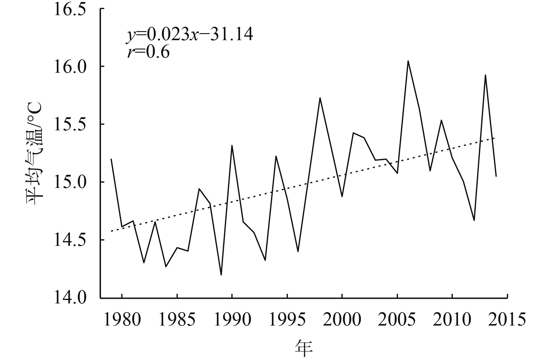
表 2 1979年—2014年三峡库区每月气温变化MK斜率和显著度
Table 2 MK trends in regional-mean temperature for each month over 1979—2014
| 月份 | 显著度 | 斜率/(℃/10 a) | 月份 | 显著度 | 斜率/(℃/10 a) |
| 1 | 0.634 | 0.014 | 7 | 0.005 | 0.389 |
| 2 | 0.070 | 0.324 | 8 | 0.577 | 0.136 |
| 3 | 0.003 | 0.626 | 9 | 0.002 | 0.448 |
| 4 | 0.026 | 0.294 | 10 | 0.236 | 0.199 |
| 5 | 0.713 | 0.094 | 11 | 0.186 | 0.144 |
| 6 | 0.153 | 0.170 | 12 | 0.454 | –0.066 |
| 注:通过5%显著性检验的以粗斜体表示。 | |||||
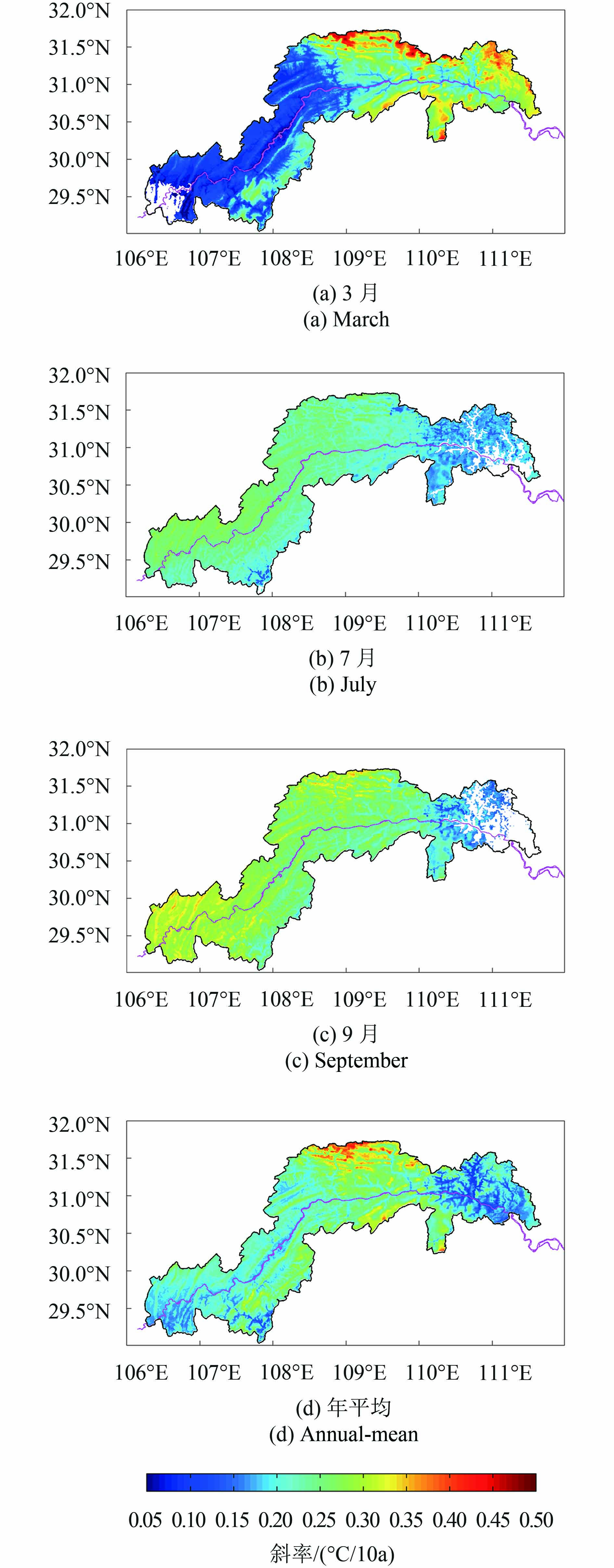
3.3 月气温变化的空间格局
本文选择了变化显著的3个月:3月、7月、9月,分别代表春、夏、秋3个季节,而后分析了3月、7月、9月及年平均气温1979年—2014年变化趋势的空间格局。从图5中可以看到,7月和9月的变化格局比较接近,西部增温速度快于东部,东部部分地区增温较慢,且很多区域的变化未达到显著水平(p>5%)。3月气温变化趋势的格局则明显与7月和9月不同,东部增温速度明显快于西部,东西分界明显,东部属于高海拔地区,其增温速度明显超过了7月和9月增温迅速的西部区域。就年均气温而言,长江中段增温速度最快,其次为西部,最慢为东部,几乎所有像素的气温增加趋势都达到了显著。
3.4 月气温动态范围的变化趋势
区域气温均值只能体现平均状态,而气候变化的表现也会表现在一些极端值上,如近期有研究发现,受极端低温明显减少的影响,美国冬季气温的数值变化范围明显缩小(Rhines 等,2017)。对此,我们提取了研究区每年每月气温分布的5%分位数(代表区域低温)和95%分位数(代表区域高温),计算其多年变化趋势(表3),从表3中可以看出如下特征。(1)区域低温增加显著的月份有:2月、3月、4月、6月、7月、9月,高温增加显著的月份有:3月、4月、7月、9月(和平均气温的计算结果一致),说明低温相对于平均气温和高温而言,变化更为显著;(2)由于多数月份低温区的增速超过了高温区的增速,导致了气温变化范围(即高温区与低温区的差值)缩小,缩小显著的是2月、3月、5月、6月。虽然在7月、8月、9月高温区的增速略微超过低温区的增速,但气温变化范围增大的趋势并不能通过显著性检验;(3)尽管3月和9月的平均气温都显著上升,但在数据上的表现是不同的,3月气温的上升主要来自于低温区的贡献,而9月的升温则更多来自高温区的贡献,这和图5(a)、5(c)的结果具有一致性。
表 3 三峡库区每月气温低温区(5%分位数)、高温区(95%分位数)、气温动态变化范围(95%与5%分位数之差)的MK变化斜率及显著度
Table 3 MK trends in low temperature (5 percentiles), high temperature (95 percentiles) and temperature range (difference between 5 percentiles and 95 percentiles) for each month
| 月份 | 5%分位数 | 95%分位数 | 动态范围 | |||||
| 显著度 | 斜率/
(℃/10 a) |
显著度 | 斜率/
(℃/10 a) |
显著度 | 斜率/
(℃/10 a) |
|||
| 1 | 0.406 | 0.080 | 0.693 | –0.099 | 0.362 | –0.179 | ||
| 2 | 0.040 | 0.401 | 0.145 | 0.253 | 0.017 | –0.149 | ||
| 3 | 0.000 | 0.809 | 0.033 | 0.477 | 0.004 | –0.332 | ||
| 4 | 0.021 | 0.335 | 0.037 | 0.285 | 0.595 | –0.050 | ||
| 5 | 0.124 | 0.243 | 0.946 | 0.002 | 0.000 | –0.240 | ||
| 6 | 0.019 | 0.285 | 0.540 | 0.099 | 0.000 | –0.186 | ||
| 7 | 0.002 | 0.357 | 0.006 | 0.415 | 0.989 | 0.058 | ||
| 8 | 0.347 | 0.122 | 0.505 | 0.182 | 0.838 | 0.060 | ||
| 9 | 0.000 | 0.431 | 0.005 | 0.490 | 0.406 | 0.058 | ||
| 10 | 0.094 | 0.232 | 0.362 | 0.197 | 0.595 | –0.035 | ||
| 11 | 0.105 | 0.222 | 0.522 | 0.052 | 0.131 | –0.170 | ||
| 12 | 0.522 | –0.067 | 0.634 | –0.096 | 0.860 | –0.029 | ||
| 注:变化显著的用加粗斜体表示。 | ||||||||
4 讨 论
4.1 气温变化趋势和海拔、森林覆盖率的关系
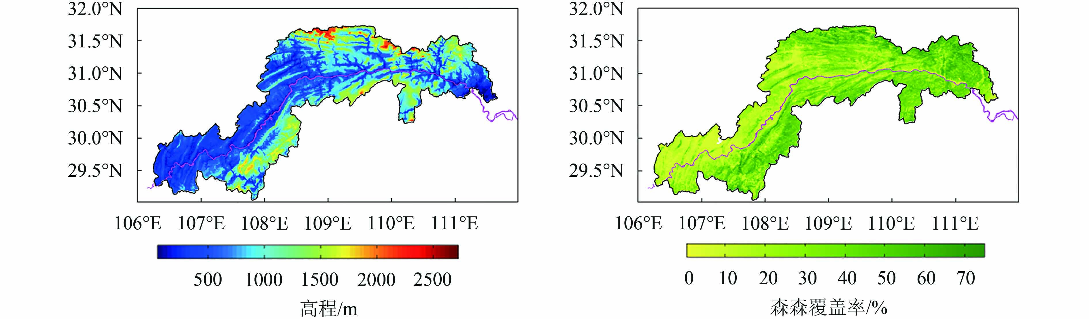
从图5(d)中可以看出,年平均温度在中部海拔较高的地区增速更快,气温增加速度和高程的相关系数达0.76,与很多研究结果相似(Diaz和Bradley,1997;Liu 等,2009)。高海拔地区环境脆弱,对气候变化敏感,经常被认为是“气候变化”的放大器(Messerli和Ives,1997),这其中的原因非常复杂,通常是由于雪盖、云量(云高)、气溶胶等变化造成的地表能量平衡的变化;此外,能量吸收随水汽含量变化的非线性特征,也会增加高海拔地区对气候变化的敏感性(Pepin 等,2015)。对于三峡地区而言,高海拔地区的增温在冬春季(3月)更显著(图5(a)),因此增温速度和高程之间的正相关极有可能与高海拔处雪盖范围和持续时间的减少有关,但这仍需要更多深入的研究。
年均温增温速度和森林覆盖率的相关系数为0.27,表面上看,森林覆盖率越高,增温速度越快,然而对于三峡库区,海拔和森林覆盖率紧密相关(两者相关系数为0.67),森林覆盖率与增温速度的正相关其实是因为他们两者都与海拔有关。为了去除海拔的干扰,分析森林对于气温变化的影响,我们计算了气温增加速度和森林覆盖率的偏相关系数(以海拔为固定因子),结果见表4。对于全年平均气温而言,偏相关系数为–0.357,说明森林覆盖率对于年均温的上升有抑制作用,对于月平均气温而言,偏相关系数存在一定季节变化。在7月—10月,森林覆盖率与增温速度呈明显负相关,可能与森林蒸散强、抑制增温有关;而在3月份,森林覆盖率与增温速度则是正相关,这可能与森林反照率变低(受雪盖减少或森林生长的影响)、吸收太阳辐射量增加有关(Li 等,2015)。
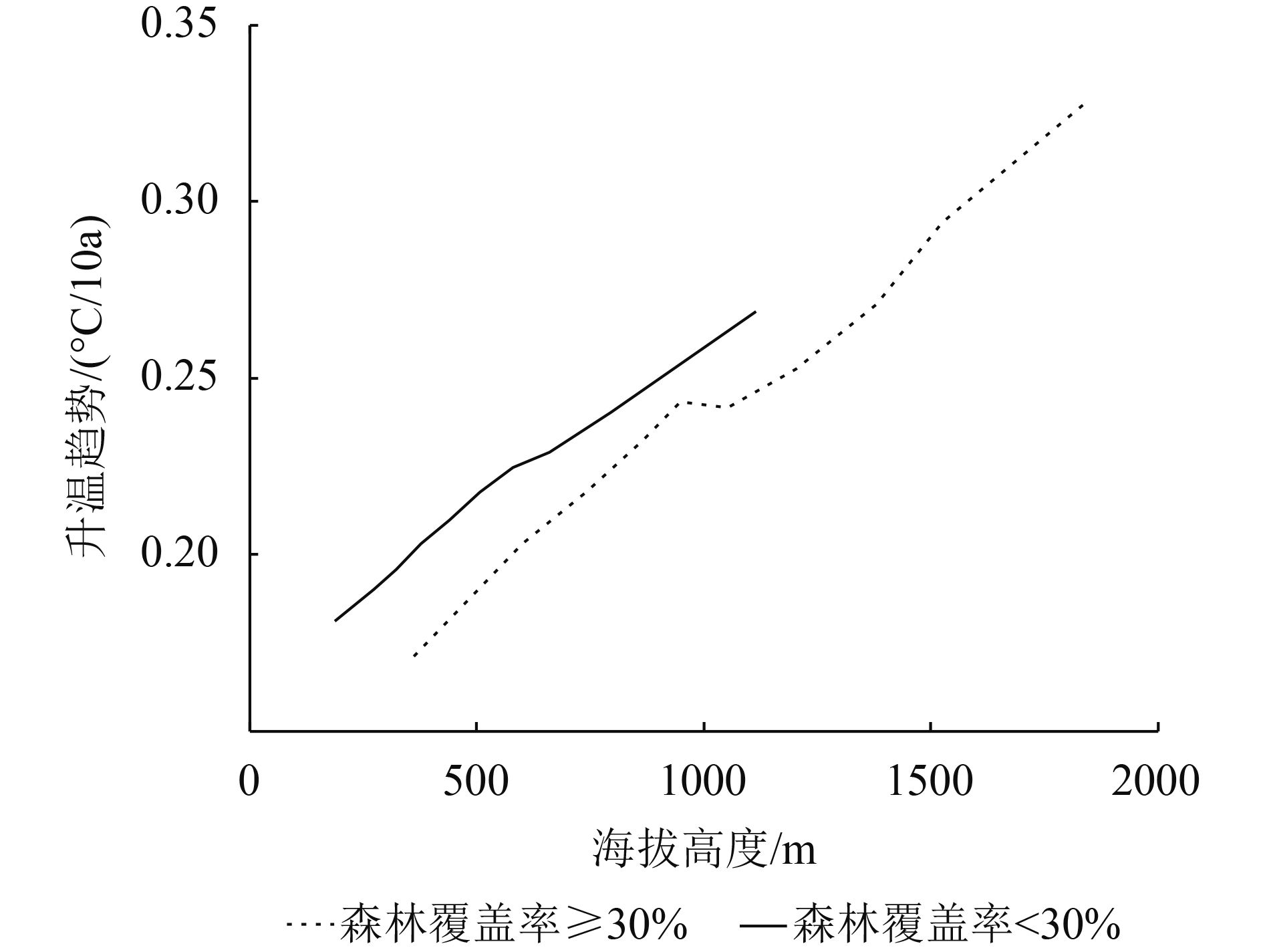
图6显示了两种不同森林覆盖度水平下海拔与年平均气温增加趋势的关系,从图6中可以看出,无论森林覆盖率高低,增温速度都随着海拔的升高而增加,但在同等海拔高度处,低森林覆盖率的增温速度高于高森林覆盖率的增温速度,暗示高覆盖率森林对增温的抑制作用在低海拔处更明显(尤其是在海拔1000 m以下区域)。
表 4 不同月份升温速率和森林覆盖率的偏相关系数(将高程作为控制因子)
Table 4 Partial correlation coefficients between temperature change trends and tree cover for each month (elevation is the control variable)
| 月份 | 升温速率和森
林覆盖率的 偏相关系数 |
月份 | 升温速率和森
林覆盖率的 偏相关系数 |
|||
| 1 | 0.084 | 8 | –0.391 | |||
| 2 | –0.383 | 9 | –0.463 | |||
| 3 | 0.319 | 10 | –0.337 | |||
| 4 | –0.274 | 11 | –0.003 | |||
| 5 | 0.041 | 12 | –0.000 | |||
| 6 | 0.217 | 平均 | –0.357 | |||
| 7 | –0.418 | |||||
4.2 气温直减率的变化
利用空间分辨率1 km的气温和高程数据,我们还可以计算气温直减率,结果如图7所示,三峡库区的年均气温直减率大约在0.49—0.56 ℃/100 m,并且存在明显的年际变化,在90年代以后,气温直减率明显下降,以1998年为界,前后两个时期年平均气温的气温直减率分别为0.53和0.51,变化达到显著(p<5%)。从前面气温百分位数和升温速率分析,可以推测年气温直减率的下降很大程度上来自冬春季节低温上升迅速的结果,低温一般出现在高海拔处,其温度的上升造成了气温垂直梯度的下降,并可能造成对流减弱,大气稳定度上升、不利于降水和污染物扩散的后果。该结果也表明,在三峡库区长时间序列气温数据的处理中,如果采用固定的气温直减率,可能会低估后期高海拔处的气温(因为实际的气温直减率在后期低于前期)。

5 结 论
本研究以GAM为插值算法,以高程和LSTnight作为辅助变量,估算了三峡库区1979年—2014年1 km空间分辨率的月气温数据。研究结果显示,气温插值精度具有明显的季节变化,在插值算法中引入LSTnight信息,可以改善气温估算精度,冬春季的改善幅度明显高于夏秋季;三峡库区的气温以上升为主,年平均温度在1997年后明显升高,但在2003年库区蓄水后变化不明显;几乎所有月(除12月)的气温都呈上升趋势,其中3月和9月的气温增加最显著;从空间格局上看,3月的增温主要位于库区东部海拔较高、森林覆盖率较大的区域,而9月的升温主要位于库区西部地形平坦、农田和城市偏多的区域,从数值上看,3月增温主要来自于低温区的快速增温,而9月增温则更大程度上来自于高温区的快速增温。多数月份(除7月、8月、9月以外)的低温区上升速度超过高温区的上升速度,导致区域温度的动态变化范围缩小,进而使得区域年均气温直减率也呈现下降趋势。
三峡库区年平均气温上升速度与高程呈正相关,即海拔越高,升温越快,但在同一海拔高度处,森林覆盖越高,年均气温的上升速度越慢,说明森林具有抑制增温的作用。数据分析结果还显示,这种抑制增温的作用在低海拔处表现得更为明显,即森林和非森林(或稀疏森林)之间气温变化速度的差异在低海拔处更大。
本文主要分析三峡库区气温的变化格局及时空分布特征,没有探讨三峡工程的影响,因为这需要考虑更大的空间范围、更多的气象要素,以及相关机理方面的解释。受人类活动的影响,森林覆盖率在1979年—2014年会发生一些变化,而本文利用了2006年的森林覆盖率数据,可能会对分析结果造成一定影响。由于森林覆盖率增加会抑制增温速率,假设在过去36年里森林覆盖率明显下降,而我们认为保持不变,则本文计算得出的升温速率应该超过完全由于气候变化造成的升温速率。未来我们将尝试评估森林覆盖率变化对区域气温变化的贡献。
参考文献(References)
-
Benali A, Carvalho A C, Nunes J P, Carvalhais N and Santos A. 2012. Estimating air surface temperature in Portugal using MODIS LST data. Remote Sensing of Environment, 124 : 108–121. [DOI: 10.1016/j.rse.2012.04.024]
-
Chen X Y, Zhang Q, Ye D X, Liao Y M, Zhu C H and Zou X K. 2009. Regional climate change over three gorges reservoir area. Resources and Environment in the Yangtze Basin, 18 (1): 47–51. [DOI: 10.3969/j.issn.1004-8227.2009.01.008] ( 陈鲜艳, 张强, 叶殿秀, 廖要明, 祝昌汉, 邹旭恺. 2009. 三峡库区局地气候变化. 长江流域资源与环境, 18 (1): 47–51. [DOI: 10.3969/j.issn.1004-8227.2009.01.008] )
-
Diaz H F and Bradley R S. 1997. Temperature variations during the last century at high elevation sites. Climate Change, 36 (3-4): 253–279. [DOI: 10.1023/A:1005335731187]
-
Hamed K H. 2008. Trend detection in hydrologic data: the Mann–Kendall trend test under the scaling hypothesis. Journal of Hydrology, 349 (3-4): 350–363. [DOI: 10.1016/j.jhydrol.2007.11.009]
-
Hill D J. 2013. Evaluation of the temporal relationship between daily min/max air and land surface temperature. International Journal of Remote Sensing, 34 (24): 9002–9015. [DOI: 10.1080/01431161.2013.860661]
-
Li X, Cheng G D and Lu L. 2003. Comparison study of spatial interpolation methods of air temperature over Qinghai-Xizang Plateau. Plateau Meteorology, 22 (6): 565–573. [DOI: 10.3321/j.issn:1000-0534.2003.06.006] ( 李新, 程国栋, 卢玲. 2003. 青藏高原气温分布的空间插值方法比较. 高原气象, 22 (6): 565–573. [DOI: 10.3321/j.issn:1000-0534.2003.06.006] )
-
Li Y, Zhao M S, Motesharrei S, Mu Q Z, Kalnay E and Li S C. 2015. Local cooling and warming effects of forests based on satellite observations. Nature Communication, 6 : 6603 [DOI: 10.1038/ncomms7603]
-
Liu X D, Cheng Z G, Yan L B and Yin Z Y. 2009. Elevation dependency of recent and future minimum surface air temperature trends in the Tibetan Plateau and its surroundings. Global and Planetary Change, 68 (3): 164–174. [DOI: 10.1016/j.gloplacha.2009.03.017]
-
Ma Z S, Zhang Q and Qin Y Y. 2010. Numerical simulation and analysis of the effect of three gorges reservoir project on the regional climate change. Resources and Environment in the Yangtze Basin, 19 (9): 1044–1052. ( 马占山, 张强, 秦琰琰. 2010. 三峡水库对区域气候影响的数值模拟分析. 长江流域资源与环境, 19 (9): 1044–1052. )
-
Messerli B and Ives J D. 1997. Mountains of the World: A Global Priority. New York: Parthenon: 495
-
Miller N, Jin J M and Tsang C F. 2005. Local climate sensitivity of the Three Gorges Dam. Geophysical Research Letters, 32 (16): L16704 [DOI: 10.1029/2005GL022821]
-
Mostovoy G V, King R L, Reddy K R, Gopal Kakani V and Filippova M G. 2006. Statistical estimation of daily maximum and minimum air temperatures from MODIS LST data over the state of Mississippi. GIScience and Remote Sensing, 43 (1): 78–110. [DOI: 10.2747/1548-1603.43.1.78]
-
Ouarda T B M J, Charron C, Marpu P R and Chebana F. 2016. The generalized additive model for the assessment of the direct, diffuse, and global solar irradiances Using SEVIRI images, with application to the UAE. IEEE Journal of Selected Topics in Applied Earth Observations and Remote Sensing, 9 (4): 1553–1566. [DOI: 10.1109/JSTARS.2016.2522764]
-
Oyler J W, Ballantyne A, Jencso K, Sweet M and Running S W. 2015. Creating a topoclimatic daily air temperature dataset for the conterminous United States using homogenized station data and remotely sensed land skin temperature. International Journal of Climatology, 35 (9): 2258–2279. [DOI: 10.1002/joc.4127]
-
Oyler J W, Dobrowski S Z, Holden Z A and Running S W. 2016. Remotely sensed land skin temperature as a spatial predictor of air temperature across the conterminous United States. Journal of Applied Meteorology and Climatology, 55 (7): 1441–1457. [DOI: 10.1175/JAMC-D-15-0276.1]
-
Park N W and Chi K H. 2008. Quantitative assessment of landslide susceptibility using high-resolution remote sensing data and a generalized additive model. International Journal of Remote Sensing, 29 (1): 247–264. [DOI: 10.1080/01431160701227661]
-
Park S. 2011. Integration of satellite-measured LST data into cokriging for temperature estimation on tropical and temperate islands. International Journal of Climatology, 31 (11): 1653–1664. [DOI: 10.1002/joc.2185]
-
Parmentier B, McGill B, Wilson A M, Regetz J, Jetz W, Guralnick R P, Tuanmu M N, Robinson N and Schildhauer M. 2014. An assessment of methods and remote-sensing derived covariates for regional predictions of 1 km daily maximum air temperature. Remote Sensing, 6 (9): 8639–8670. [DOI: 10.3390/rs6098639]
-
Pepin N, Bradley R S, Diaz H F, Baraer M, Caceres E B, Forsythe N, Fowler H, Greenwood G, Hashmi M Z, Liu X D, Miller J R, Ning L, Ohmura A, Palazzi E, Rangwala I, Schöner W, Severskiy I, Shahgedanova M, Wang M B, Williamson S N and Yang D Q. 2015. Elevation-dependent warming in mountain regions of the world. Nature Climate Change, 5 (5): 424–430. [DOI: 10.1038/NCLIMATE2563]
-
Ren Z H and Xiong A Y. 2007. Operational system development on three step quality control of observations from AWS. Meteorological Monthly, 33 (1): 19–24. [DOI: 10.7519/j.issn.1000-0526.2007.01.003] ( 任芝花, 熊安元. 2007. 地面自动站观测资料三级质量控制业务系统的研制. 气象, 33 (1): 19–24. [DOI: 10.7519/j.issn.1000-0526.2007.01.003] )
-
Rhines A, McKinnon K A, Tingley M P and Huybers P. 2017. Seasonally resolved distributional trends of north American temperatures show contraction of winter variability. Journal of Climate, 30 (3): 1139–1157. [DOI: 10.1175/JCLI-D-16-0363.1]
-
Tietäväinen H, Tuomenvirta H and Venäläinen A. 2010. Annual and seasonal mean temperatures in Finland during the last 160 years based on gridded temperature data. International Journal of Climatology, 30 (15): 2247–2256. [DOI: 10.1002/joc.2046]
-
Vancutsem C, Ceccato P, Dinku T and Connor S J. 2010. Evaluation of MODIS land surface temperature data to estimate air temperature in different ecosystems over Africa. Remote Sensing of Environment, 114 (2): 449–465. [DOI: 10.1016/j.rse.2009.10.002]
-
Wan Z, Zhang Y, Zhang Q and Li Z L. 2004. Quality assessment and validation of the MODIS global land surface temperature. International Journal of Remote Sensing, 25 (1): 261–274. [DOI: 10.1080/0143116031000116417]
-
Wang Y Y, Guo Z, Li G C and Guo Z D. 2017. Precipitation estimation and analysis of the Three Gorges Dam region (1979—2014) by combining gauge measurements and MSWEP with generalized additive model. Acta Geographica Sinica, 72 (7): 1207–1220. [DOI: 10.11821/dlxb201707007] ( 王圆圆, 郭徵, 李贵才, 郭兆迪. 2017. 基于广义加性模型估算1979—2014年三峡库区降水及其特征分析. 地理学报, 72 (7): 1207–1220. [DOI: 10.11821/dlxb201707007] )
-
Wood S N. 2003. Thin plate regression splines. Journal of the Royal Statistical Society Series B (Statistical Methodology), 65 (1): 95–114. [DOI: 10.1111/1467-9868.00374]
-
Wu J, Gao X J, Giorgi F, Chen Z H and Yu D F. 2012. Climate effects of the three Gorges Reservoir as simulated by a high resolution double nested regional climate model. Quaternary International, 282 : 27–36. [DOI: 10.1016/j.quaint.2012.04.028]
-
Wu L G, Zhang Q and Jiang Z H. 2006. Three Gorges Dam affects regional precipitation. Geophysical Research Letters, 33 (13): L13806 [DOI: 10.1029/2006GL026780]
-
Yu Q, Peng N Z and Fu B P. 1996. A preliminary study on climatic characteristics and cause of formation in three gorges. Journal of Lake Science, 8 (4): 305–311. [DOI: 10.18307/1996.0403] ( 于强, 彭乃志, 傅抱璞. 1996. 三峡气候的基本特征和成因的初步研究. 湖泊科学, 8 (4): 305–311. [DOI: 10.18307/1996.0403] )
-
Zhang Q, Wan S Q, Mao Y W, Chen Z H and Liao Y M. 2005. Characteristics of temperature changes around the Three Gorges with complex topography. Advances in Climate Change Research, 1 (4): 164–167. [DOI: 10.3969/j.issn.1673-1719.2005.04.005] ( 张强, 万素琴, 毛以伟, 陈正洪, 廖要明. 2005. 三峡库区复杂地形下的气温变化特征. 气候变化研究进展, 1 (4): 164–167. [DOI: 10.3969/j.issn.1673-1719.2005.04.005] )
-
Zhang T Y, Fan L, Sun J, He Y K, Dong X N and Ren Y J. 2010. Characteristics of climate change in the three gorges reservoir area during 1961~2008. Resources and Environment in the Yangtze Basin, 19 (S1): 52–61. ( 张天宇, 范莉, 孙杰, 何永坤, 董新宁, 任永建. 2010. 1961~2008年三峡库区气候变化特征分析. 长江流域资源与环境, 19 (S1): 52–61. )
-
Zhang X T, Liang S L, Song Z, Niu H L, Wang G X, Tang W J, Chen Z Q and Jiang B. 2016. Local adaptive calibration of the satellite-derived surface incident shortwave radiation product using smoothing spline. IEEE Transactions on Geoscience and Remote Sensing, 54 (2): 1156–1169. [DOI: 10.1109/TGRS.2015.2475615]
-
Zhao F and Shepherd M. 2012. Precipitation changes near Three Gorges Dam, China. Part I: a spatiotemporal Validation Analysis. Journal of Hydrometeorology, 13 (2): 735–745. [DOI: 10.1175/JHM-D-11-061.1]
-
Zhou Y and Yuan J K. 2016. Analysis of temperature variation before and after impoundment of Three Gorges reservoir. Meteorological Science and Technology, 44 (5): 783–787. [DOI: 10.3969/j.issn.1671-6345.2016.05.015] ( 周英, 袁久坤. 2016. 三峡库区" 腹心”地带蓄水前后气温变化特征. 气象科技, 44 (5): 783–787. [DOI: 10.3969/j.issn.1671-6345.2016.05.015] )