|
收稿日期: 2016-04-21; 优先数字出版日期: 2017-09-01
基金项目: 国家重点基础研究发展计划(973计划)(编号:2013CB733406,2013CB733404);国家高技术研究发展计划(863计划)(编号:2012AA 12A306);中央高校基本科研业务费专项资金(编号:2015KJJCA12);中央级公益性科研院所基本科研业务费专项资金项目(编号:CAFYBB2016ZD004)
第一作者简介: 蒙诗栎(1990— ),女,博士研究生,研究方向为遥感影像处理和林业遥感。E-mail:mengsl@mail.bnu.edu.cn
通讯作者简介: 庞勇(1976— ),男,研究员,研究方向为主动遥感机理建模与森林参数定量反演、森林生物量和碳储量计量。E-mail:pangy@ifrit.ac.cn
中图分类号: TP701
文献标识码: A
|
摘要
使用高空间分辨率卫星WorldView-2的多光谱遥感影像,构建植被指数和纹理因子等遥感因子与森林地上生物量的关系方程,并计算模型估测精度和均方根误差,探索高分辨率数据的光谱与纹理信息在温带森林地上生物量估测应用中的潜力。以黑龙江省凉水自然保护区温带天然林及天然次生林为研究对象,通过灰度共生矩阵(GLCM)、灰度差分向量(GLDV)及和差直方图(SADH)对高分辨率遥感影像进行纹理信息提取,并利用外业调查的74个样地地上生物量与遥感因子建立参数估计模型。提取的遥感因子包括6种植被指数(比值植被指数RVI、差值植被指数DVI、规一化植被指数NDVI、增强植被指数EVI、土壤调节植被指数SAVI和修正的土壤调节植被指数MSAVI)以及3类纹理因子(GLCM、GLDV和SADH)。为避免特征变量个数较多对估测模型造成过拟合,利用随机森林算法对提取的遥感因子进行特征选择,将最优的特征变量输入模型参与建模估测。采用支持向量回归(SVR)进行生物量建模及验证,结果显示选入模型的和差直方图均值(sadh_mean)、灰度共生矩阵方差(glcm_var)和差值植被指数(DVI)等遥感因子对森林地上生物量有较好的解释效果;植被指数+纹理因子组合的模型获得较精确的AGB估算结果(R2=0.85,RMSE=42.30 t/ha),单独使用植被指数的模型精度则较低(R2=0.69,RMSE=61.13 t /ha)。
关键词
地上生物量, 纹理因子, WorldView-2, 高分辨率遥感影像, 温带森林, 随机森林, 支持向量回归
Abstract
The effect of forest biomass on carbon cycles has long been recognized.Therefore, an accurate assessment of forest biomassis required to understand ecosystem changes. This research uses vegetation indices and textural indices based on high spatial resolution Worldview-2 multispectral imagery to establish their relationship with forest AGB (Above Ground Biomass) and assess the accuracy of the estimation model. This research also explores the capability of spectral and textural information for AGB assessment at the Liang Shui National Nature Reserve, Northeast China. Remote sensing vegetation and texture indices were derived from high spatial resolution Worldview-2 multispectral data. We applied three different algorithms to extract the texture indices from the Worldview-2 data, including Gray Level Co-occurrence Matrix, Gray Level Difference Vector, and Sum and Difference Histograms. Six vegetation indices, namely, RVI, DVI, NDVI, EVI, SAVI, and MSAVI, were computed. The relationship among the above mentioned indices and 74 field measurements was established.However, the over fitting problems for the training regression model could occur due to the many input independent variables (i.e., vegetation indices and texture indices), which could decrease the robustness of the regression model. The random forest algorithm could avoid overfitting through the training process, so it was utilized to perform feature selection. Several optimal variables were selected to conduct the regression analysis.The support vector regression method was implemented to train and validate the AGB models. Results show that variables selection could better interpret forest AGB and obtain accurate predicted results. Comparisons between the two estimation models were made. The first model only applied vegetation indices, whereas the other model integrated vegetation and texture indices. The results also show that the accuracy of the vegetation indices model was lower than the vegetation+textural indices model (integrated vegetation indices with texture indices) at R2=0.69, RMSE=61.13 t/ha and R2=0.85, RMSE=42.30 t/ha, respectively. This research confirms that textural information could improve the accuracy of forest AGB estimation to a certain extent.
Key words
aboveground biomass, texture indices, WorldView-2, high spatial resolution remote sensing image, temperate forest, random forest, SVR
1 引 言
森林生态系统作为陆地生态系统中最重要的生态系统之一,在全球碳循环、控制温室气体以及维持地球生物圈的稳定中占有举足轻重的地位。世界各国正在加强合作,扩大森林面积,促进可持续森林经营,提高森林质量,增加碳汇以应对全球气候变化。精确估算森林蓄积量以及地上生物量AGB(Aboveground Biomass)是评估生态系统过程、碳平衡及气候变化的一个重要基础(Roy和Ravan,1996)。
与传统的实地勘察测量的方法不同,利用遥感技术可以快速、准确、无破坏的对森林生物量进行估算,且易于从林分尺度推广到大面积区域的森林,尤其对一些地面测量难以进行的偏远地区的天然林来说,遥感技术的优势更加突显。在较大区域甚至全球尺度上实现对森林蓄积的变化与监测,遥感技术仍是目前应用最为广泛的方法(Hyde,2006)。微波遥感具有极强的穿透能力,如合成孔径雷达SAR(Synthetic Aperture Radar)能与森林生物量的主体即树干和树枝发生作用而广泛运用于估算森林AGB(Dobson 等,1992;Foody 等,1997;Mitchard 等,2009),然而SAR信号受地形起伏影响较大,且当生物量达到一定水平时后向散射系数趋于饱和(陈尔学,1999),因此在森林结构复杂的高生物量地区其应用具有一定局限性。激光雷达LiDAR(Light Detection and Ranging)在林木高度测量和森林垂直结构信息获取方面具有其他遥感技术无可比拟的优势(Nelson 等,1988;Lefsky 等,1999;Patenaude 等,2004;Bortolot和Wynne,2005),且高精度的激光雷达森林参数反演结果还可用作其他遥感产品的验证数据(庞勇 等,2005),但LiDAR数据由于覆盖区域有限、花费昂贵、数据量大等特点限制了其在大面积森林中的应用(马利群和李爱农,2011)。光学传感器仍是估算森林生物量研究中普遍使用且较为可靠的数据获取源(Foody 等,2001;Fuchs 等,2009;Lu, 2005; Muukkonen和Heiskanen,2007)。中等空间分辨率数据如Landsat TM(Thematic Mapper)和ETM+(Enhanced Thematic Mapper Plus)(Zheng 等,2004;Labrecque 等,2006;Avitabile 等,2012)广泛用于区域和全球尺度的森林生物量估测研究,而其有限的描绘细节能力无法得到更精细尺度上的生物量变化。
随着各类星载、机载传感器技术和搭载平台的不断更新与发展,高分辨率光学影像的获取更加便捷,各商业卫星产品空间分辨率更是达到米级甚至亚米级别,如SPOT 5(2.5 m全色,10 m多光谱),IKONOS(1.0 m全色,4.0 m多光谱),GF-2(0.8 m全色,3.2 m多光谱),QuickBird(0.65 m全色,2.62 m多光谱),WorldView-2(0.46 m全色,1.84 m多光谱),GeoEye-1(0.41 m全色,1.65 m多光谱)和WorldView-3(0.31 m全色,1.24 m多光谱)等。高分辨率光学遥感影像可以充分利用光谱信息、植被指数信息、纹理信息以及空间特征反映更详细的森林遥感信息(李德仁 等,2012),在森林结构参数研究方面有巨大潜力。
估算森林生物量通常使用的遥感因子包括波段反射率、波段比、植被指数等光谱衍生因子。使用光谱因子的局限在于,对森林类型丰富、冠层封闭且生物量水平较高的热带及亚热带地区,由于光谱信息饱和较难得到高预测精度(Franklin和Mcdermid,1993;Hyyppä 等,2000)。影像纹理信息作为遥感影像的派生数据,由于其揭示了图像内容的水平结构信息并反映图像灰度值空间变化规律和空间相关特性,逐渐被加入到生物量估算模型中。在光学及SAR影像数据中加入纹理因子参与估算生物量,模型精度均能有效提升(Franklin 等,2000;Nelson 等,2000;Podest和Saatchi,2002;Dekker,2003;Lu和Batistella,2005;Sarker,2011),同时,纹理因子被广泛应用于土地覆盖分类和其他森林结构参数的估测如年龄、密度、叶面积指数等(Cohen和Spies,1992;Podest和Saatchi,2002;Champion 等,2008)。
本研究选择3种纹理提取算法用于测试纹理因子对AGB估算的能力,分别是灰度共生矩阵GLCM(Gray Level Co-occurrence Matrix)、灰度差分矢量GLDV(Gray Level Difference Vector)及和差直方图SADH(Sum and Difference Histogram)。GLCM表示在给定窗口范围内根据设定的间隔和方向统计相邻灰度出现的频数(Haralick 等,1973),是计算纹理常用的方法之一(柳钦火 等,2010);GLDV基本思路来源于GLCM,它描述的是在给定窗口范围内相邻灰度值的绝对差值的概率分布,GLCM和GLDV在遥感分类和参数提取研究中使用较为普遍(李智峰 等,2011;Sarker,2011),SADH(Unser,1986)作为常规共生矩阵的替代,描述影像中特定间隔与方向上相邻灰度之间和与差的概率分布。然而,纹理是一种复杂属性,高度依赖于被研究对象、采用的窗口大小及地形状况,且计算纹理会产生大量数据(Franklin 等,2000;Marceau 等,1990)。
WorldView-2数据在森林树种分类(Rapinel 等,2014;Heenkenda 等,2014)和湿地生物量估测(Mutanga 等,2012)方面的研究均取得较好的效果,而WorldView-2数据对森林结构复杂和高值生物量地区的研究仍存在较多不确定因素。本研究通过对WorldView-2高分辨率多光谱数据提取植被指数以及纹理因子,利用随机森林算法对植被指数、GLCM纹理因子、SADH纹理因子以及GLDV纹理因子进行特征选择,并通过支持向量回归SVR(Support Vector Regression)算法建立生物量估测模型,比较植被指数以及采用植被指数+纹理因子相结合的两种情况下模型的预测潜力,为提高森林生物量的定量反演精度提供参考。
2 研究区及数据
2.1 研究区
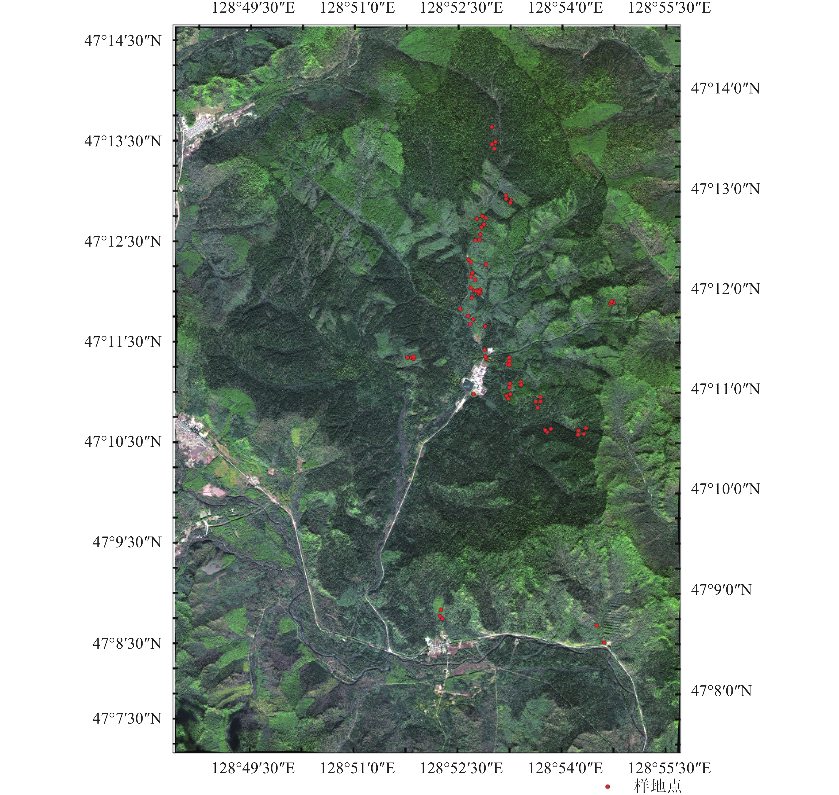
实验研究区(图1)位于中国东北部黑龙江省伊春市带岭区凉水国家级自然保护区(47°10′N,128°53′E)。凉水自然保护区地处小兴安岭南坡达里带岭支脉的东坡,海拔高度在280—707 m,是典型的低山丘陵地貌。保护区面积约为1.2万hm2,森林总蓄积量170万m3,区内植被群落类型复杂多样,是中国现存较大面积的原始红松林之一。保护区以原始红松林为主,还有主要保护对象是以红松为主的温带针阔叶混交林,伴生多种温性阔叶树种,如糠椴、枫桦、蒙古柞、大青杨、裂叶榆、五角槭等。另外还伴生一些寒温性针叶树种,如红皮云杉、鱼鳞云杉、臭冷杉等;同时林内有发育良好的山葡萄、五味子、狗枣猕猴桃等藤本植物(马建章 等,1993;刘吉春 等,1993)。

2.2 遥感数据
WorldView-2多光谱影像获取时间为2010年9月29日,空间分辨率为2 m。卫星传感器提供8个波段数据,其中包括4个标准波段:蓝、绿、红、近红外(NIR1)及4个非标准波段:海岸、黄、红边、近红外2(NIR2)(表1),文中仅探讨4个标准波段对AGB的估测能力。首先对WorldView-2数据进行辐射定标得到辐亮度数据,利用ENVI 5.0软件(The Environment for Visualizing Images,Exelis Visual Information Solutions Inc.,Boulder, CO, USA)的基于MODTRAN4+模型的FLAASH模块对辐亮度数据进行大气校正,得到遥感反射率影像。根据Digital Global公司对WorldView-2产品的描述信息,影像精准度具有6.5 m水平误差,小于4.1 m垂直误差(无需控制点状态)。在利用样地定位影像前先将数据产品进行几何校正,从1∶10000尺度地形图上选取35个地面控制点对WorldView-2多光谱影像进行配准,经几何精校正后位置总误差小于0.86个像元。
表 1 WorldView-2多光谱数据光谱信息
Table 1 The spectral information of WorldView-2 multispectral data
| 波段 | 像素大小/nm | 波长范围/nm | 中心波长/nm |
| 全色 | 0.5 | 450—800 | 625 |
| 海岸 | 2 | 400—450 | 425 |
| 蓝 | 2 | 450—510 | 480 |
| 绿 | 2 | 510—580 | 545 |
| 黄 | 2 | 585—625 | 605 |
| 红 | 2 | 630—690 | 660 |
| 红边 | 2 | 705—745 | 725 |
| 近红外 | 2 | 770—895 | 835 |
| 近红外2 | 2 | 860—1040 | 950 |
2.3 样地数据
地面调查工作于2009年7月26日至8月14日开展,根据森林类型和不同蓄积量等级高、中、低,每个梯度分别抽取3—4个森林区划小班布设样地,共采集78个圆形样地,半径为13.8 m,与黑龙江省森林资源清查样地面积保持一致,基本覆盖了针叶、阔叶和针阔混交等森林类型(庞勇和李增元,2012)。测量了样地内所有胸径DBH(Diameter at Breast Height)大于5 cm的单木,记录胸径、树高、枝下高、冠幅、树种等测树因子。胸径通过PI卷尺测量,树高和枝下高使用激光测高仪测量(TruPulse 360B,Laser Technology Inc.,Centennial CO,USA),冠幅采用皮尺测量。各测树因子统计直方图如图2所示。胸径分布的偏度最大,存在少部分胸径较大的单木(>40 cm),冠幅、树高与枝下高分布较分散,略接近于正态分布。通过分树种异速生长模型计算每株检尺木的地上生物量Wa、活枝生物量Wb、叶生物量Wf、根生物量Wt、树干生物量Ws和总生物量Wt,通过每木组分生物量累加得到样地尺度上的组分生物量,进而换算成单位面积的组分生物量(t/hm2)。主要树种的组分生物量异速生长方程参见陈传国和朱俊凤(1989)和Wang(2006),样地生物量模型拟合R2均大于0.8(庞勇和李增元,2012)。样地中心经纬坐标使用差分全球定位系统DGPS(Difference Global Positioning System)确定,其中4块样地未能进行差分处理,本研究仅使用有差分GPS坐标的74块样地,经差分处理后位置误差小于1 m(样地信息详见附录)。
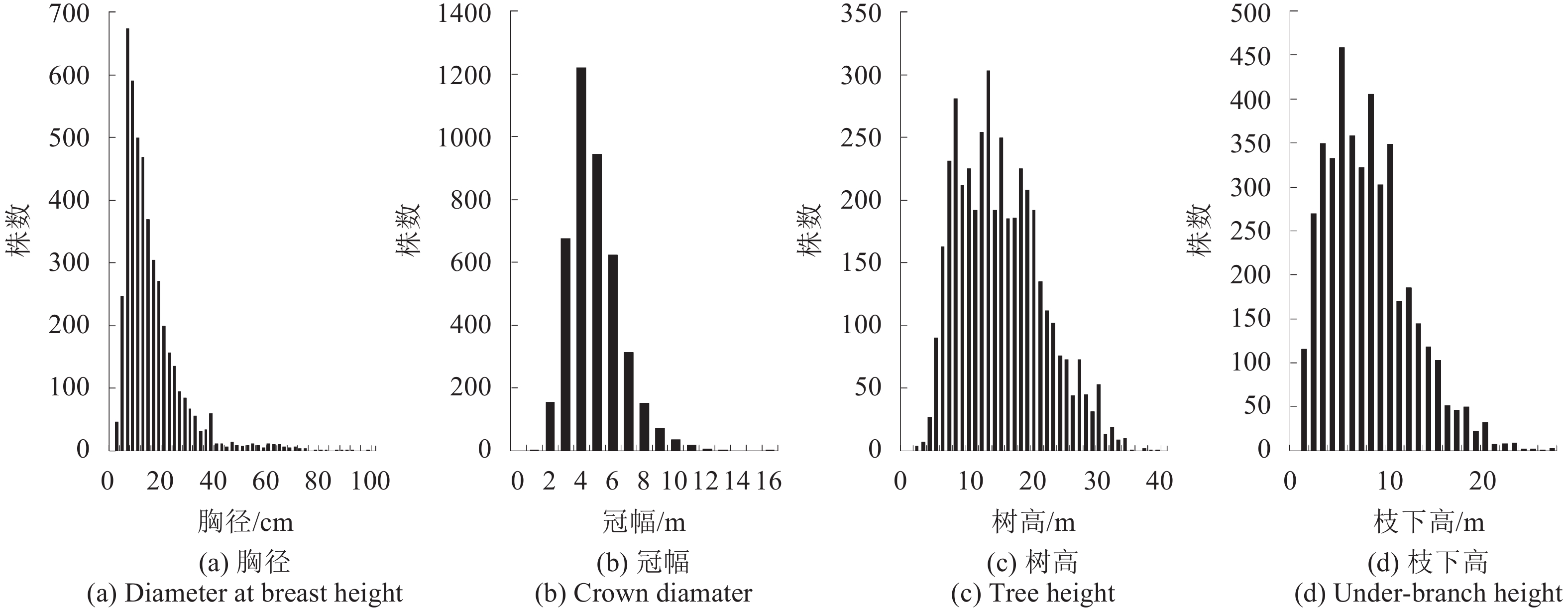
表 A1 样地坐标和地上生物量信息
Table A1 Information of coordinate and AGB for sample plots
| ID | 经纬度 | 生物量/(t/ha) | ID | 经纬度 | 生物量/(t/ha) | |
| 1 | 128.8964°E, 47.1768°N | 357.06 | 38 | 128.8974°E, 47.1773°N | 283.11 | |
| 2 | 128.8876°E, 47.1831°N | 178.01 | 39 | 128.9039°E, 47.1770°N | 315.22 | |
| 3 | 128.8867°E, 47.1828°N | 203.79 | 40 | 128.9038°E, 47.1763°N | 277.17 | |
| 4 | 128.8937°E, 47.1819°N | 226.93 | 41 | 128.8960°E, 47.1771°N | 352.61 | |
| 5 | 128.8948°E, 47.1826°N | 444.54 | 42 | 128.9057°E, 47.1774°N | 412.03 | |
| 6 | 128.8871°E, 47.1823°N | 190.40 | 43 | 128.9053°E, 47.1765°N | 303.25 | |
| 7 | 128.8942°E, 47.1808°N | 333.22 | 44 | 128.8901°E, 47.1851°N | 121.47 | |
| 8 | 128.8949°E, 47.1818°N | 360.09 | 45 | 128.8874°E, 47.1842°N | 130.59 | |
| 9 | 128.8837°E, 47.2238°N | 271.69 | 46 | 128.8814°E, 47.1904°N | 72.49 | |
| 10 | 128.8831°E, 47.2245°N | 337.36 | 47 | 128.8902°E, 47.1846°N | 173.19 | |
| 11 | 128.8817°E, 47.2046°N | 74.119 | 48 | 128.8875°E, 47.1848°N | 120.77 | |
| 12 | 128.8839°E, 47.2249°N | 308.33 | 49 | 128.8816°E, 47.1893°N | 79.11 | |
| 13 | 128.8829°E, 47.2274°N | 260.09 | 50 | 128.8788°E, 47.2002°N | 115.41 | |
| 14 | 128.8803°E, 47.2004°N | 55.53 | 51 | 128.8799°E, 47.1997°N | 85.81 | |
| 15 | 128.8816°E, 47.2123°N | 137.60 | 52 | 128.8781°E, 47.2007°N | 131.37 | |
| 16 | 128.8812°E, 47.2112°N | 161.04 | 53 | 128.8793°E, 47.2002°N | 100.76 | |
| 17 | 128.8865°E, 47.2161°N | 329.98 | 54 | 128.8786°E, 47.1955°N | 81.24 | |
| 18 | 128.8877°E, 47.2151°N | 251.09 | 55 | 128.8755°E, 47.1972°N | 71.73 | |
| 19 | 128.8795°E, 47.2121°N | 110.51 | 56 | 128.8803°E, 47.1998°N | 53.94 | |
| 20 | 128.8808°E, 47.2126°N | 163.16 | 57 | 128.8775°E, 47.2054°N | 99.26 | |
| 21 | 128.8865°E, 47.2155°N | 275.38 | 58 | 128.8780°E, 47.2049°N | 93.18 | |
| 22 | 128.8876°E, 47.2148°N | 194.99 | 59 | 128.8779°E, 47.1947°N | 61.98 | |
| 23 | 128.8803°E, 47.2095°N | 73.24 | 60 | 128.8774°E, 47.1960°N | 112.97 | |
| 24 | 128.8802°E, 47.2087°N | 161.82 | 61 | 128.8799°E, 47.2001°N | 24.54 | |
| 25 | 128.8785°E, 47.2031°N | 113.89 | 62 | 128.8784°E, 47.2031°N | 109.35 | |
| 26 | 128.8791°E, 47.2020°N | 83.80 | 63 | 128.8781°E, 47.2025°N | 86.69 | |
| 27 | 128.8806°E, 47.2108°N | 138.27 | 64 | 128.8874°E, 47.1885°N | 91.67 | |
| 28 | 128.8791°E, 47.2086°N | 94.48 | 65 | 128.8868°E, 47.1881°N | 107.44 | |
| 29 | 128.8782°E, 47.1991°N | 104.04 | 66 | 128.8873°E, 47.1891°N | 112.58 | |
| 30 | 128.8815°E, 47.1943°N | 96.36 | 67 | 128.8874°E, 47.1879°N | 112.27 | |
| 31 | 128.9102°E, 47.1419°N | 49.25 | 68 | 128.8628°E, 47.1891°N | 74.72 | |
| 32 | 128.8707°E, 47.1463°N | 36.73 | 69 | 128.8638°E, 47.1891°N | 97.03 | |
| 33 | 128.8710°E, 47.1473°N | 43.89 | 70 | 128.9124°E, 47.1983°N | 68.84 | |
| 34 | 128.8818°E, 47.1889°N | 161.39 | 71 | 128.8644°E, 47.1889°N | 85.36 | |
| 35 | 128.9084°E, 47.1447°N | 155.05 | 72 | 128.8643°E, 47.1893°N | 94.19 | |
| 36 | 128.8713°E, 47.1458°N | 26.86 | 73 | 128.9117°E, 47.1981°N | 48.93 | |
| 37 | 128.8787°E, 47.1831°N | 39.44 | 74 | 128.9119°E, 47.1985°N | 58.83 |
3 方 法
基于WorldView-2数据的4个标准波段提取植被指数,同时分别计算3种类型纹理因子(GLCM、GLDV与SADH)。经过对提取的遥感因子进行变量选择,将筛选出的对回归模型影响力较大的变量因子进行SVR回归,构建出凉水自然保护区的森林生物量预测模型。研究方法由3部分组成,提取光谱及纹理等遥感特征、特征选择和SVR回归建模。
3.1 提取遥感特征
根据样地点中心的地理坐标,将样地坐标作为中心像元,对15×15窗口内的像元值取平均作为遥感提取的特征,得出WorldView-2影像的植被指数及纹理信息。研究中采用的6种植被指数详见表2。
表 2 植被指数计算公式
Table 2 Equations for vegetation indices
| 植被指数 | 公式 | 参考文献 |
| 比值植被指数RVI (Ratio Vegetation Index) |
|
Pearson和Miller,1972 |
| 差值植被指数DVI (Difference Vegetation Index) |
|
Richardson和Weigand,1977 |
| 归一化植被指数NDVI (Normalized Difference Vegetation Index) |
|
Rouse 等,1974 |
| 增强植被指数EVI (Enhanced Vegetation Index) |
|
Liu和Huete,1995 |
| 土壤调节植被指数SAVI (Soil Adjusted Vegetation Index) |
|
Huete,1988 |
| 修正的土壤调节植被指数MSAVI (Modified Soil Adjusted Vegetation Index) |
|
Qi 等,1994 |
| 注:B,R,NIR1分别代表Worldview-2影像蓝、红、近红外波段反射率;EVI中的系数为C1=6.0,C2=7.5,C3=1,G=2.5(Colombo 等,2003);SAVI中L设置为0.5。 | ||
提取的影像纹理因子包括8个GLCM纹理因子、7个SADH纹理因子和5个GLDV纹理因子。各类纹理因子计算公式详见表3。计算纹理时所选择的窗口大小是影响灰度统计矩阵特征的因素之一,本研究选取不同窗口大小(7×7,9×9,11×11,13×13,15×15,17×17)计算森林纹理特征值,分析不同窗口下各纹理因子对AGB的预测能力。3类纹理特征均采用默认的0°方向和1个像元统计间隔。
表 3 本研究采用的纹理因子
Table 3 Textural parameters utilized in this research
| 计算方法 | 纹理因子 | 公式 |
| 灰度共生矩阵(GLCM) | 均值 (mean) |
|
| 方差 (variance) |
|
|
| 均匀性 (homogeneity) |
|
|
| 对比度 (contrast) |
|
|
| 异质性 (dissimilarity) |
|
|
| 熵 (entropy) |
|
|
| 二阶矩 (secondary moment) |
|
|
| 相关性 (correlation) |
|
|
| 和差直方图(SADH) | 均值 (mean) |
|
| 方差 (variance) |
|
|
| 能量 (energy) |
|
|
| 相关性 (correlation) |
|
|
| 熵 (entropy) |
|
|
| 对比度 (contrast) |
|
|
| 均匀性 (homogeneity) |
|
|
| 灰度差分向量(GLDV) | 均值 (mean) |
|
| 方差 (variance) |
|
|
| 能量 (energy) |
|
|
| 对比度 (contrast) |
|
|
| 二阶矩 (secondary moment) |
|
|
| 注:Pij为归一化共生矩阵,ME为灰度共生矩阵的均值; |
||
3.2 特征选择
随机森林算法(Breiman,2001)是一种准确率高且鲁棒性较好的机器学习算法,适合处理高维且特征高度相关的数据集。算法原理为利用bootstrap方法从原始样本中有放回地多次重复随机抽取,对每次抽取的样本进行决策树建模,通过组合多棵决策树的预测,最终经投票得出预测结果。R软件(R Development Core Team,2009)提供的Random Forest程序包可对变量进行特征选择。通过判断自变量在回归过程中对因变量的影响力从而评估该自变量对回归模型的重要性。影响力的评价通过两个指标来实现,一是自变量出现在袋外数据OOBD(Out Of Bag Data)时的模型均方差增量百分数%IncMSE(Increase Mean Squared Error%),二是自变量出现在OOBD时对模型树节点纯度的影响力(node purity),由残差平方和来衡量。当某一自变量出现在OOBD时,其模型MSE增量越高,则表示回归模型对该自变量的需求度越高,即加入该自变量能有效减少模型估测误差。反之当自变量出现在OOBD时模型MSE增量较低,则将该变量加入模型时对整体估算精度影响不大。
3.3 SVR回归建模
SVR是支持向量机SVM(Support Vector Machine)算法在回归中的应用。通过选择合适的核函数将样本从低维空间转换到高维空间,使得低维空间内的非线性问题可在高维空间中线性处理,并保证良好的泛化能力。Libsvm(Chang和Lin,2011)是一个功能强大的免费工具箱,对SVM涉及的参数调整较少并提供参数寻优和交叉验证的功能,可解决分类和回归等问题。Libsvm可在指定的区间内进行格网化寻优,得出经交叉验证后回归精度最优的惩罚系数C和径向基核函数RBF(Radical Basis Fuction)的参数gamma,并利用该最优参数回归模型实现对森林AGB的预测和反演。
4 实验结果
4.1 自变量因子特征选择结果
采用随机森林算法对WorldView-2影像的植被指数以及7×7,9×9,11×11,13×13,15×15,17×17窗口内计算的纹理因子与植被指数组合进行特征选择。将所有变量按照对模型的重要性进行排序,选择删除比例为二分之一,从当前特征变量中剔除不重要的变量;再用新特征集合建立新的随机森林,逐个计算新特征变量的重要性;重复迭代上述步骤,直到剩下特征数目为样本个数的10%至20%。最后一次迭代中特征变量对回归模型的重要性排序结果如图3所示,按照从高到低顺序分别列出各特征出现在OOBD时的模型增量%IncMSE。图3(a)—(f)为植被指数+纹理因子组合不同窗口下的重要变量因子,图3(g)为植被指数的模型增量%IncMSE排序。
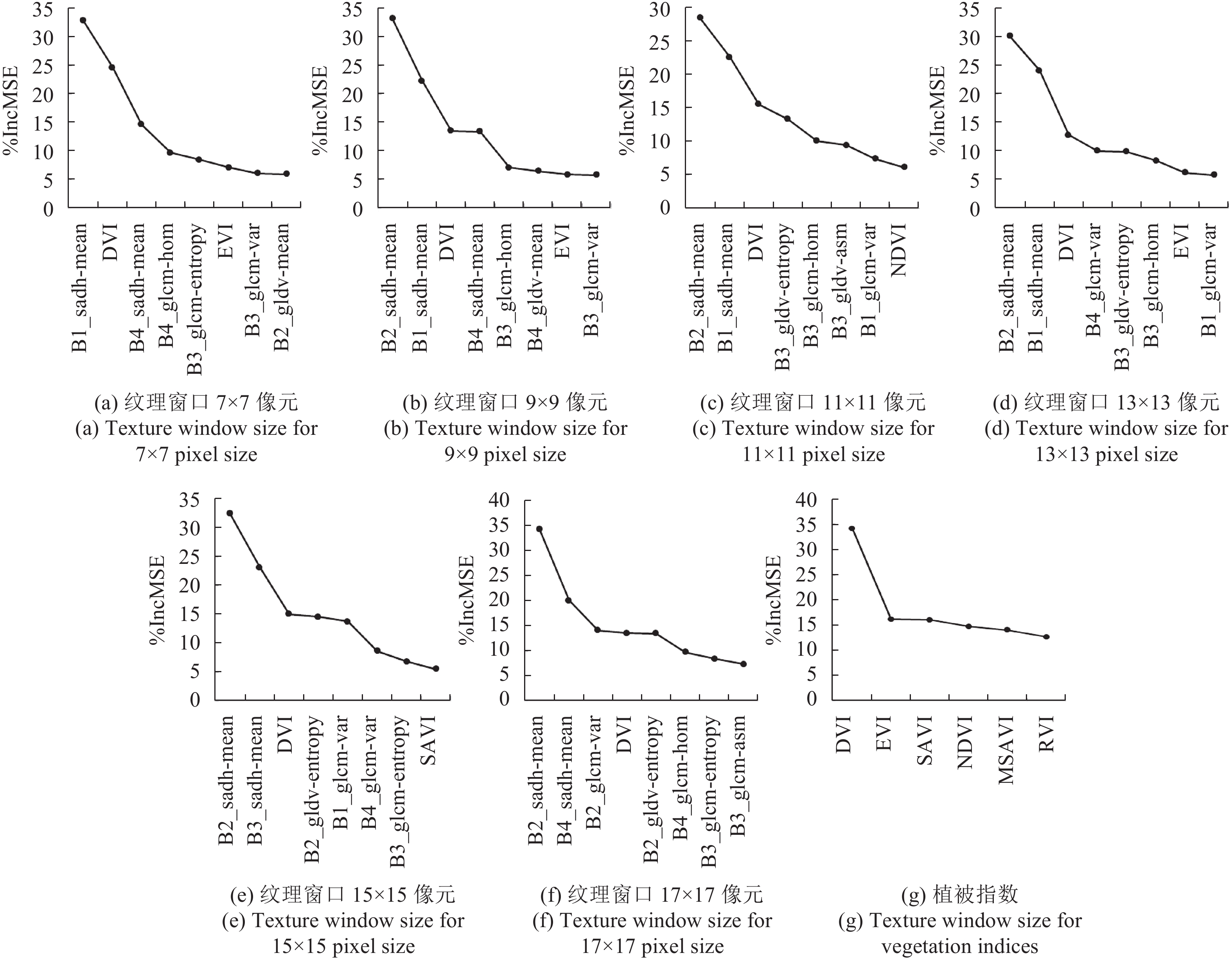
特征变量按照变量重要性排序,越往后重要性越低曲线趋势逐渐平缓。对于6种不同窗口的光谱—纹理综合的特征排序,前8个遥感因子的特征对于模型贡献十分重要,其中B2_sadh_mean(绿波段SADH纹理的均值因子)特征出现在OOBD时回归模型增量%IncMSE均高于25%,光谱—纹理组合中光谱特征DVI的贡献也较高,不同窗口下的%IncMSE均大于10%。DVI在植被指数中对模型的重要性达34.6%,远高于其余植被指数特征。光谱—纹理组合第8个变量之后的特征对模型重要性较低,则加入变量对估测精度影响不大,因此本文采用前8个变量对AGB进行回归建模。对于光谱特征,文中采用前3个变量进行AGB回归。
4.2 植被指数和植被指数+纹理因子回归建模结果
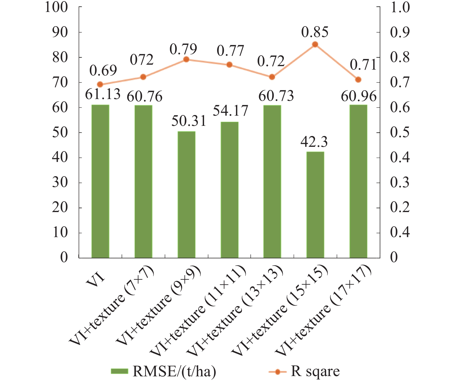
经过对从WorldView-2数据中提取的遥感因子进行特征选择,将对模型贡献大的变量与样地AGB进行SVR回归,通过Libsvm进行参数寻优得出精度最佳的预测模型。图4为植被指数以及6种不同窗口的植被指数(VI)+纹理因子(texture)与样地AGB的建模结果。可看出,采用植被指数与纹理特征相结合的方式进行AGB回归建模的精度明显优于仅采用植被指数建模的精度,表现为前者的R2较高且RMSE较低。仅采用植被指数与AGB拟合时精度为最低(R2=0.69,RMSE=61.13 t/ha),植被指数+纹理因子结合与AGB的拟合效果相比之均较高。其中,不同统计窗口内的纹理模型估测精度也不同。15×15窗口提取的纹理与植被指数组合与生物量相关性最好,模型R2高达0.85,其RMSE也最低,为42.30 t/ha。
4.3 研究区AGB预测
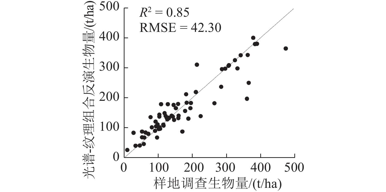
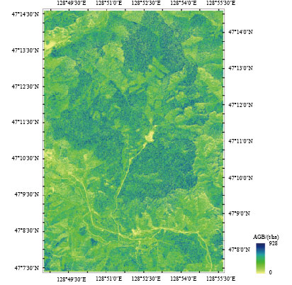
最优回归模型的“留一法”交叉验证结果显示(图5),遥感数据提取的植被指数+纹理因子组合与样地实测生物量相关性较好,预测精度高(R2=0.85,RMSE=42.30 t/ha,rRMSE%=24.31%)。将SVR的最优回归模型即15×15窗口提取的纹理—光谱组合的模型对凉水地区完整覆盖的WorldView-2影像进行AGB反演(图6),图中除极少数由于光谱噪声等导致的异常高值区域(>600 t/ha)外,估测生物量的均值±1倍的标准差为237.42±131.13 t/ha。
4.4 讨论
研究表明,单独使用植被指数不足以建立高精度的生物量预测模型。且由于其对郁闭度和生物量水平较高的地区易产生光谱信息饱和,较难对上述地区的森林生物量进行准确预估。纹理的贡献提高了生物量估测模型的精度,从图4看出,植被指数对生物量的预测能力(R2=0.69,RMSE=61.13 t/ha)弱于加入纹理信息后的预测能力(R2=0.71—0.85,RMSE=42.30—60.96 t/ha)。在变量选择中波段反射率的均值纹理因子都会被首先选入,通过一定窗口(如15×15窗口)的平均,可以在一定程度上降低椒盐噪声的影响。在纹理计算过程中,窗口大小的选择对纹理因子提取结果和回归模型精度有较大影响,最优的窗口尺寸是影像空间分辨率和林木冠幅的一个综合。窗口较小时,窗口内每个像元灰度值对纹理因子的贡献度更大,单个树冠内部的差异对纹理因子的贡献也会加大;窗口过大时则提取结果更大程度上反应了过多森林冠层或地形起伏等方面的大尺度纹理特征,无法有效描述森林冠层纹理信息。WorldView-2影像分辨率较高,较小窗口7×7或9×9的纹理信息对冠层的解释性弱于15×15,更大的窗口尺寸提取的纹理信息则会趋向于刻画大尺度的特征。纹理随所用影像及地表特征不同而变化,挑选与生物量相关性强、与其他变量相关性弱的纹理因子较为困难。有效的纹理判定通过窗口大小选择、影像波段选择和适当的纹理提取算法等方面决定,再经过回归分析得出精度较高的预测模型。
从图5散点图得出,在生物量较小水平上(<100 t/ha)遥感预测结果普遍略高于实测数据,在较高生物量水平上(>300 t/ha)得到遥感预测结果略低于实测数据,该现象表明估算生物量时的饱和现象并不能完全消除,但加入了有效的遥感特征能减弱信号饱和带来的影响。高分辨率遥感影像的纹理特征十分丰富,通过加入纹理信息,使植被指数+纹理因子组合估测模型的精度(R2=0.85,RMSE=42.30 t/ha)显著高于仅使用植被指数的精度(R2=0.69,RMSE=61.13 t/ha)。且图6显示,生物量预测结果(237.42±131.13 t/ha)与Meng等人(2016)采用激光雷达百分位数进行高精度生物量反演的统计结果相似(245.27±92.91 t/ha),表明基于纹理特征的反演算法可行且结果可靠。
在回归模型建模过程中,若将某些对因变量影响不大甚至没有影响的自变量加入回归模型,不仅会给运算增加负担,同时模型的预测结果和估计精度也会下降。在本研究中,回归模型的特征变量个数(86个)多于地面调查的样本个数(74个),将全部变量输入模型参与回归则会增加模型过拟合的风险,即对训练样本拟合非常好,对测试样本的应用效果很差。因此,在进行模型回归前通常先对变量因子进行特征选择。好的特征选择算法能提升模型性能,使模型泛化能力更强,减少过拟合,同时增强对特征和特征值的互相理解。基于随机森林的变量筛选的方法能选出有效且数目更少的变量因子(Díaz-Uriarte和de Andrés,2006),其选出的变量通常具有最小的袋外误差(out of bag error)(Stumpf和Kerle,2011)。
5 结 论
本研究主要探究利用WorldView-2高分辨率多光谱影像的光谱和纹理特征对森林生物量的估算潜力,采用了GLCM、GLDV和SADH等算法计算纹理因子,并将纹理因子与植被指数相结合与样地生物量进行回归建模。对比实验结果表明加入纹理因子对提高生物量模型的估测精度有一定贡献,尤其是可以提高生物量高值区域的估测精度。在变量特征选择过程中引入随机森林算法,从全体特征变量中剔除不重要的变量直到剩下的重要特征个数为样本个数的10%至20%。该数值为经过测试后确定的经验比例,如何根据特定模型自适应确定合理的变量个数需要进一步研究。
参考文献(References)
-
Avitabile V, Baccini A, Friedl M A and Schmullius C. 2012. Capabilities and limitations of Landsat and land cover data for aboveground woody biomass estimation of Uganda. Remote Sensing of Environment, 117 : 366–380. [DOI: 10.1016/j.rse.2011.10.012]
-
Bortolot Z J and Wynne R H. 2005. Estimating forest biomass using small footprint LiDAR data: an individual tree-based approach that incorporates training data. ISPRS Journal of Photogrammetry and Remote Sensing, 59 (6): 342–360. [DOI: 10.1016/j.isprsjprs.2005.07.001]
-
Breiman L. 2001. Random forests. Machine Learning, 45 (1): 5–32. [DOI: 10.1023/A:1010933404324]
-
Champion I, Dubois-Fernandez P, Guyon D and Cottrel M. 2008. Radar image texture as a function of forest stand age. International Journal of Remote Sensing, 29 (6): 1795–1800. [DOI: 10.1080/01431160701730128]
-
Chang C C and Lin C J. 2011. LIBSVM: a library for support vector machines[EB/OL]. http://www.csie.ntu.edu.tw/~cjlin/libsvm
-
Chen C G and Zhu J F. 1989. Woody Biomass Manual of Typical Species in the Northeast of China. Beijing: China Forestry Publishing House (陈传国, 朱俊凤. 1989. 东北主要林木生物量手册. 北京: 中国林业出版社)
-
Chen E X. 1999. Development of forest biomass estimation using SAR data. World Forestry Research, 12 (6): 18–23. [DOI: 10.3969/j.issn.1001-4241.1999.06.004] ( 陈尔学. 1999. 合成孔径雷达森林生物量估测研究进展. 世界林业研究, 12 (6): 18–23. [DOI: 10.3969/j.issn.1001-4241.1999.06.004] )
-
Cohen W B and Spies T A. 1992. Estimating structural attributes of douglas-fir/western hemlock forest stands from landsat and SPOT imagery. Remote Sensing of Environment, 41 (1): 1–17. [DOI: 10.1016/0034-4257(92)90056-P]
-
Colombo R, Bellingeri D, Fasolini D and Marino C M. 2003.Retrieval of leaf area index in different vegetation types using high resolution satellite data. Remote Sensing of Environment, 86(1): 120–131
-
Díaz-Uriarte R and de Andrés S A. 2006. Gene selection and classification of microarray data using random forest. BMC Bioinformatics, 7: 3 [DOI: 10.1186/1471-2105-7-3]
-
Dekker R J. 2003. Texture analysis and classification of ERS SAR images for map updating of urban areas in the Netherlands. IEEE Transactions on Geoscience and Remote Sensing, 41 (9): 1950–1958. [DOI: 10.1109/TGRS.2003.814628]
-
Dobson M C, Ulaby F T, LeToan T, Beaudoin A, Kasischke E S and Christensen N. 1992. Dependence of radar backscatter on coniferous forest biomass. IEEE Transactions on Geoscience and Remote Sensing, 30 (2): 412–415. [DOI: 10.1109/36.134090]
-
Foody G M, Cutler M E, Mcmorrow J, Pelz D, Tangki H, Boyd D S and Douglas I. 2001. Mapping the biomass of Bornean tropical rain forest from remotely sensed data. Global Ecology and Biogeography, 10 (4): 379–387. [DOI: 10.1046/j.1466-822X.2001.00248.x]
-
Foody G M, Green R M, Lucas R M, Curran P J, Honzak M and Do Amaral I. 1997. Observations on the relationship between SIR-C radar backscatter and the biomass of regenerating tropical forests. International Journal of Remote Sensing, 18 (3): 687–694. [DOI: 10.1080/014311697219024]
-
Franklin S E, Hall R J, Moskal L M, Maudie A J and Lavigne M B. 2000. Incorporating texture into classification of forest species composition from airborne multispectral images. International Journal of Remote Sensing, 21 (1): 61–79. [DOI: 10.1080/014311600210993]
-
Franklin S E and McDermid G J. 1993. Empirical relations between digital SPOT HRV and CASI spectral response and lodgepole pine (Pinus contorta) forest stand parameters. International Journal of Remote Sensing, 14 (12): 2331–2348. [DOI: 10.1080/01431169308954040]
-
Fuchs H, Magdon P, Kleinn C and Flessa H. 2009. Estimating aboveground carbon in a catchment of the Siberian forest tundra: combining satellite imagery and field inventory. Remote Sensing of Environment, 113 (3): 518–531. [DOI: 10.1016/j.rse.2008.07.017]
-
Haralick R M, Shanmugam K and Dinstein I H. 1973. Textural features for image classification. IEEE Transactions on Systems, Man, and Cybernetics, SMC-3 (6): 610–621. [DOI: 10.1109/TSMC.1973.4309314]
-
Heenkenda M K, Joyce K E, Maier S W and Bartolo R. 2014. Mangrove species identification: comparingWorldView-2 with aerial photographs. Remote Sensing, 6 (7): 6064–6088. [DOI: 10.3390/rs6076064]
-
Huete A R. 1988. A soil-adjusted vegetation index (SAVI). Remote Sensing of Environment, 25 (3): 295–309. [DOI: 10.1016/0034-4257(88)90106-X]
-
Hyde P, Dubayah R, Walker W, Blair J B, Hofton M and Hunsaker C. 2006. Mapping forest structure for wildlife habitat analysis using multi-sensor (LiDAR, SAR/InSAR, ETM+, Quickbird) synergy. Remote Sensing of Environment, 102 (1): 63–73.
-
Hyyppä J, Hyyppä H, Inkinen M, Engdahl M, Linko S and Zhu Y H. 2000. Accuracy comparison of various remote sensing data sources in the retrieval of forest stand attributes. Forest Ecology and Management, 128 (1/2): 109–120. [DOI: 10.1016/S0378-1127(99)00278-9]
-
Labrecque S, Fournier R A, Luther J E and Piercey D. 2006. A comparison of four methods to map biomass from Landsat-TM and inventory data in western Newfoundland. Forest Ecology and Management, 226 (1/3): 129–144. [DOI: 10.1016/j.foreco.2006.01.030]
-
Lefsky M A, Harding D, Cohen W B, Parker G and Shugart H H. 1999. Surface Lidar remote sensing of basal area and biomass in deciduous forests of eastern Maryland, USA. Remote Sensing of Environment, 67 (1): 83–98. [DOI: 10.1016/S0034-4257(98)00071-6]
-
Li D R, Wang C W, Hu Y M and Liu S G. 2012. General review on remote sensing-based biomass estimation. Geomatics and Information Science of Wuhan University, 37 (6): 631–635. ( 李德仁, 王长委, 胡月明, 刘曙光. 2012. 遥感技术估算森林生物量的研究进展. 武汉大学学报(信息科学版), 37 (6): 631–635. )
-
Li Z F, Zhu G C and Dong T F. 2011. Application of GLCM-based texture features to remote sensing image classification. Geology and Exploration, 47 (3): 456–461. ( 李智峰, 朱谷昌, 董泰锋. 2011. 基于灰度共生矩阵的图像纹理特征地物分类应用. 地质与勘探, 47 (3): 456–461. )
-
Liu H Q and Huete A. 1995. A feedback based modification of the NDVI to minimize canopy background and atmospheric noise. IEEE Transactions on Geoscience and Remote Sensing, 33 (2): 457–465. [DOI: 10.1109/36.377946]
-
Liu J C, Liu B W and Zhang P. 1993. Scientific value and advantage of LiangShui nature conservation area. Journal of wildlife, (1): 4-5 (刘吉春, 刘伯文, 张鹏. 1993. 凉水自然保护区的科研价值与优势. 野生动物, (1): 4–5)
-
Liu Q H, Xin X Z, Tang P, Liao J J and Wu B F. 2010. Research on Quantitative Remote Sensing Model, Application and Uncertainty. Beijing: Science Press (柳钦火, 辛晓洲, 唐娉, 廖静娟, 吴炳方. 2010. 定量遥感模型、应用及不确定性研究. 北京: 科学出版社)
-
Lu D. 2005. Aboveground biomass estimation using Landsat TM data in the Brazilian Amazon. International Journal of Remote Sensing, 26 (12): 2509–2525. [DOI: 10.1080/01431160500142145]
-
Lu DS and Batistella M. 2005. Exploring TM image texture and its relationships with biomass estimation in Rondônia, Brazilian Amazon. Acta Amazonica, 35 (2): 249–257. [DOI: 10.1590/S0044-59672005000200015]
-
Ma J Z, Liu C Z and Zhang P. 1993. Research of Liang Shui Nature Conservation. Harbin: Northeast Forestry University Press (马建章, 刘传照, 张鹏. 1993. 凉水自然保护区研究. 哈尔滨: 东北林业大学出版社)
-
Ma L Q and Li A N. 2011. Review of application of LiDAR to estimation of forest vertical structure parameters. World Forestry Research, 24 (1): 41–45. ( 马利群, 李爱农. 2011. 激光雷达在森林垂直结构参数估算中的应用. 世界林业研究, 24 (1): 41–45. )
-
Marceau D J, Howarth P J, Dubois J M and Gratton D J. 1990. Evaluation of the grey-level co-occurrence matrix method for land-cover classification using SPOT imagery. IEEE Transactions on Geoscience and Remote Sensing, 28 (4): 513–519. [DOI: 10.1109/TGRS.1990.572937]
-
Meng S L, Pang Y, Zhang Z J, Jia W and Li Z Y. 2016. Mapping aboveground biomass using texture indices from aerial photos in a temperate forest of northeastern China. Remote Sensing, 8 (3): 230 [DOI: 10.3390/rs8030230]
-
Mitchard E T A, Saatchi S S, Woodhouse I H, Nangendo G, Ribeiro N S, Williams M, Ryan C M, Lewis S L, Feldpausch T R and Meir P. 2009. Using satellite radar backscatter to predict above-ground woody biomass: a consistent relationship across four different African landscapes. Geophysical Research Letters, 36 (23): L23401 [DOI: 10.1029/2009GL040692]
-
Mutanga O, Adam E and Cho MA. 2012. High density biomass estimation for wetland vegetation usingworldview-2 imagery and random forest regression algorithm. International Journal of Applied Earth Observation and Geoinformation, 18 : 399–406. [DOI: 10.1016/j.jag.2012.03.012]
-
Muukkonen P and Heiskanen J. 2007. Biomass estimation over a large area based on standwise forest inventory data and ASTER and MODIS satellite data: a possibility to verify carbon inventories. Remote Sensing of Environment, 107 (4): 617–624. [DOI: 10.1016/j.rse.2006.10.011]
-
Nelson R, Krabill W and Tonelli J. 1988. Estimating forest biomass and volume using airborne laser data. Remote Sensing of Environment, 24 (2): 247–267. [DOI: 10.1016/0034-4257(88)90028-4]
-
Nelson R F, Kimes D S, Salas W A and Routhier M. 2000. Secondary forest age and tropical forest biomass estimation using thematic mapper imagery: single-year tropical forest age classes, a surrogate for standing biomass, cannot be reliably identified using single-date tm imagery. Bioscience, 50 (5): 419–431. [DOI: 10.1641/0006-3568(2000)050[0419:sfaatf]2.0.co;2]
-
Pang Y and Li Z Y. 2012. Inversion of biomass components of the temperate forest using airborne Lidar technology in Xiaoxing’an Mountains, northeastern of China. Chinese Journal of Plant Ecology, 36 (10): 1095–1105. [DOI: 10.3724/SP.J.1258.2012.01095] ( 庞勇, 李增元. 2012. 基于机载激光雷达的小兴安岭温带森林组分生物量反演. 植物生态学报, 36 (10): 1095–1105. [DOI: 10.3724/SP.J.1258.2012.01095] )
-
Pang Y, Li Z Y, Chen E X and Sun G Q. 2005. Lidar remote sensing technology and its application in forestry. Scientia Silvae Sinicae, 41 (3): 129–136. [DOI: 10.3321/j.issn:1001-7488.2005.03.022] ( 庞勇, 李增元, 陈尔学, 孙国清. 2005. 激光雷达技术及其在林业上的应用. 林业科学, 41 (3): 129–136. [DOI: 10.3321/j.issn:1001-7488.2005.03.022] )
-
Patenaude G, Hill R A, Milne R, Gaveau D L A, Briggs B B J and Dawson T P. 2004. Quantifying forest above ground carbon content using LiDAR remote sensing. Remote Sensing of Environment, 93 (3): 368–380. [DOI: 10.1016/j.rse.2004.07.016]
-
Pearson R L and Miller L D. 1972. Remote mapping of standing crop biomass for estimation of the productivity of the shortgrass prairie//Proceedings of the Eighth International Symposium on Remote Sensing of Environment.Ann Arbor, Michigan, USA: [s.n.]: 1355
-
Podest E and Saatchi S. 2002. Application of multiscale texture in classifying JERS-1 radar data over tropical vegetation. International Journal of Remote Sensing, 23 (7): 1487–1506. [DOI: 10.1080/01431160110093000]
-
Qi J, Chehbouni A, Huete A R, Kerr Y H and Sorooshian S. 1994. A modified soil adjusted vegetation index. Remote Sensing ofEnvironment, 48 (2): 119–126. [DOI: 10.1016/0034-4257(94)90134-1]
-
R Development Core Team. 2009. R: A Language and Environment for Statistical Computing. Vienna, Austria: R Foundation for Statistical Computing
-
Rapinel S, Clément B, Magnanon S, Sellin V and Hubert-Moy L. 2014. Identificationand mapping of natural vegetation on a coastal site using aWorldview-2 satellite image. Journal of Environmental Management, 144 : 236–246. [DOI: 10.1016/j.jenvman.2014.05.027]
-
Richardson A J amd Wiegand C L.. 1977. Distinguishing vegetation from soil background information. Photogrammetric Engineering and Remote Sensing, 43 (12): 1541–1552.
-
Rouse Jr J W, Haas R H, Schell J A and Deering D W. 1974. Monitoring Vegetation Systems in the Great Plains with Erts. [s.l.]: NASA Special Publication, 351: 309
-
Roy P S and Ravan S A. 1996. Biomass estimation using satellite remote sensing data-an investigation on possible approaches for natural forest. Journal of Biosciences, 21 (4): 535–561. [DOI: 10.1007/BF02703218]
-
Sarker M L R. 2011. Estimation of Forest Biomass Using Remote Sensing.Hong Kong: Hong Kong Polytechnic University
-
Stumpf A and Kerle N. 2011. Object-oriented mapping of landslides using random forests. Remote Sensing of Environment, 115 (10): 2564–2577. [DOI: 10.1016/j.rse.2011.05.013]
-
Unser M. 1986. Sum and difference histograms for texture classification. IEEE Transactions on Pattern Analysis and Machine Intelligence, PAMI-8 (1): 118–125. [DOI: 10.1109/TPAMI.1986.4767760]
-
Wang C K. 2006. Biomass allometric equations for 10 co-occurring tree species in Chinese temperate forests. Forest Ecology and Management, 222 (1/3): 9–16. [DOI: 10.1016/j.foreco.2005.10.074]
-
Zheng D, Rademacher J, Chen J, Crow T, Bresee M and Le Moine J. 2004. Estimating aboveground biomass using Landsat 7 ETM+ data across a managed landscape in northern Wisconsin, USA. Remote Sensing of Environment, 93 (3): 402–411. [DOI: 10.1016/j.rse.2004.08.008]