 2016, Vol. 30
The Chinese Meteorological Society
Article Information
- GAO Shouting, ZHOU Feifan, ZUO Qunjie . 2016.
- The Mesoscale Balance and Imbalance and the Corresponding Potential Vorticity Inversion from the View of Helicity. 2016.
- J. Meteor. Res., 30(4): 559-571
- http://dx.doi.org/10.1007/s13351-016-5115-1
Article History
- Received December 15, 2015
- in final form July 1, 2016


The balance and imbalance in the meteorology usually refer to the relationship between wind and mass. It is noted that this relationship does not vary with time. However, the wind or mass can change with time. Thus, it is a kind of dynamic balance. The imbalance is related to the degree that the physical variables depart from the balance. In meteorology, the common balances are the static balance and the geostrophic balance. The basic states of all the synoptic systems satisfy the static balance. Actually, the geostrophic balance is hard to satisfy. But the quasigeostrophic approximation, semigeostrophic approximation, and geostrophic momentum approximation, which are all based on geostrophic balance, become the popular approximations to be used in studying largescale atmospheric motions, fronts, and jets(Allen et al., 1990; Xu, 1994; Liu and Sun, 2000; Ding, 2005). However, strong mesoscale convective systems always present as static imbalance. Meanwhile, due to their evident nongeostrophic features, the quasigeostrophic approximation cannot be adopted in mesoscale systems. Although semigeostrophic approximation and geostrophic momentum approximation can be used in some mesoscale systems(e.g., the fronts and jets), as far as other mesoscale systems with strong divergence or convergence or without band structure(such as the mesoscale convective system)are concerned, those approximations cannot be used.
The nonlinear balance equation and the corresponding balance models were developed simultaneously with the abovementioned approximations. They can also be used to explain different weather systems with different assumptions.
Charney(1955, 1962)was the first person who gave the nonlinear balance equation. It was deduced with the assumption that Rossby number is very small and thus it is just fit for largescale systems. Raymond(1992)deduced the nonlinear balance equation with a large Rossby number, and with the assumption that the velocity potential, divergence, and the vertical velocity are all very small. The finally obtained nonlinear balance equation is like Eq.(3)in Section 2, but with a different presentation of the pressure gradient force(including the nondimensional parameter π). Obviously, it is not applicable to the mesoscale systems with strong convergence or divergence. Similar to the nonlinear balance equation, the balance equations with different forms such as quasibalance, linear balance, bilinear balance, semibalance, close balance, and hybrid balance equations have been proposed(Allen et al., 1990; Barth et al., 1990; Xu, 1994). All these equations are obtained from the simplification of divergence equation. They adopted Rossby number Ro< 1, or supposed that some terms are much small and thus can be ignored(such as the divergence and convergence terms, the vertical velocity, and velocity potential terms). The above balance equations can be used in largescale weather systems or the mesoscale shallow convective systems. However, they cannot be used in the mesoscale systems that possess strong divergent or convergent winds. Another kind of balance equation is the slow equation(Lynch, 1989). It is obtained by the combination of vorticity equation and continuity equation, while the time tendency term in the combination is ignored. While this slow equation keeps the divergent effect, it is based on the barotropic model and considers the motion of largescale vortex. Therefore, the slow equation is also in the scope of geostrophic balance, and it is not suitable for mesoscale systems. Thus, some scholars argued that the mesoscale system lacks balance(Doswell III, 1987).
However, the observations and simulations on the MCS and mesoscale convective complex(MCC) showed that there exists mesoscale convective vortex(MCV)(Leary and Rappaport, 1987; Zhang and Fritsch, 1988; Brandes, 1990; Houez et al., 1991; Fritsch et al., 1994). The MCV has a warm center similar to the tropical cyclone, which enhances the inertial stabilization and makes the diabatic heating more effective on producing balance rotating flow. Previous studies showed that these flows are in balance and their thermodynamic structure varies with the mesoscale circulation. Thus, we think that there are balanced motions in the mesoscale system, and there should be corresponding describable equations. Considering that during many mesoscale systems' evolutions, the vortex plays an important role in the mesoscale system's sustainment and development(Xu, 1994; Cao and Xu, 2011; Deng and Zhou, 2011; Fu et al., 2011, 2015). It is supposed that the vortex is also the most important in mesoscale balance, but here the divergent effect can no longer be ignored. Thus, in mesoscale systems, the balance equation should contain both the rotational and divergent winds. In addition, the vertical motion is also very important in the mesoscale system, which should be included in the mesoscale balance equation. Because it is hard to describe the mesoscale balance motions in the abovementioned balance equations, in this paper, we deduce a new balance equation from the helicity equation that is capable of accommodating the divergent and rotational winds simultaneously.
The structure of this paper is as follows. Section 2 reviews the quasigeostrophic balance and imbalance. Then, analysis of helicity equation and the subsequent deductions of mesoscale balance equation and mesoscale imbalance equation are given in Section 3. The mesoscale balance models and their related potential vorticity(PV)inversion are presented in Section 4. Finally, the utility of the mesoscale balance models and the prospect of its related PV inversion are discussed in Section 5.
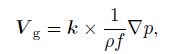
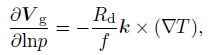
2 The quasigeostrophic balance and imbalanceThe largescale motion is quasigeostrophic. It satisfies the following geostrophic balance and thermal balance(Holton, 2004).
|
(1) |
|
(2) |
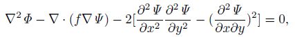
where Vg is the geostrophic wind, k indicates the vertical direction, ρ is the atmospheric density, f is the Coriolis parameter, p is the pressure, T is the temperature, and Rd is the gas constant of dry air. A nonlinear balance equation is first presented by Charney(1955, 1962), which can be written as
|
(3) |
where Φ is the geopotential and Ψ is stream function. The p coordinate is used, and there is 

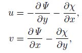
If divergence wind is considered in the total wind, there is
|
where χ is the potential function. Supposing Ro is very small, Allen et al.(1990)gave the following nonlinear balance equation:
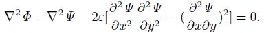
|
(4) |
If the small terms whose magnitudes are in the second order of ε(denoted by O(ε2))are also kept, the nonlinear balance equation becomes
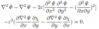
|
(5) |
The above balance equations are all supposing that Ro(or ε)< 1, namely, the Coriolis force is more important than the inertial force. However, in the mesoscale system, as we know, the Coriolis, inertial, and pressure gradient forces are comparable. Their total effect determines the development of the mesoscale system. Thus, Eqs.(3)-(5)are just fit for largescale systems.
The balance model is a series of equations that are constructed based on balance equation. It is noted that besides the balance equation, a slow time tendency equation should be included in the balance model. Of course, there can be static equation, thermodynamic equation, vorticity equation, continuity equation, etc. The largescale quasigeostrophic approximation, semigeostrophic approximation, and geostrophic momentum approximation are actually balance models. Balance model can be used to de scribe both the balance motion and the variation fea tures of the dynamic balance.
The largescale imbalance motion refers to the motions that do not satisfy the geostrophic balance, thermal wind balance, or nonlinear balance. There are corresponding diagnostic tools to analyze the imbalance motion. The most direct way is taking the divergent equation as the imbalance equation. The sum of the balance terms is first calculated, as well as the sum of the remained terms. The two sums are then compared to diagnose the imbalance(Moore and Abeling, 1988). Meanwhile, the divergence and vertical velocity are taken as reference.
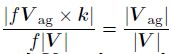
Besides, there are several tools to diagnose the largescale imbalance flows(Zhang et al., 2000). The
first one is the Lagrangian Rossby number. It is defined by Hoskins(1975)as 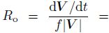
The third one is the ω equation. The ω equation in p coordinate under the adiabatic and frictionless conditions can be presented as $\sigma {{\nabla }^{2}}\omega +f_{0}^{2}\frac{{{\partial }^{2}}\omega }{\partial {{p}^{2}}}={{f}_{0}}\frac{\partial }{\partial p}\left[ {{V}_{\text{g}}}\cdot \nabla \left( {{f}_{0}}{{\nabla }^{2}}\phi +f \right) \right]+{{\nabla }^{2}}\left[ {{V}_{\text{g}}}\cdot \nabla \left( -\frac{\partial \phi }{\partial p} \right) \right]$. Here σ is the hydrostatic stability parameter, f = f0 + βy, f0 is the Coriolis parameter at the corresponding latitude, β = df /dy = const, and φ is the geopotential height. The first term on the right hand side of the equation indicates the difference of the advection of absolute vorticity at each level. The second term indicates the advection of temperature. If the value of the first term is larger than 0, ascending appears, and vice versa. For example, the first term in the downstream of a trough is usually larger than 0, thus there are ascendings in the downstream of the trough. Correspondingly, there are usually decendings in the downstream of a ridge. Besides, warm advection indicates ascending, while cold advection indicates decending. The forcing of the vertical motions can be analyzed by the righthand side terms. The fourth tool is the inverse of the PV. Its idea is that the inverse of the PV can give the variables that are in balance, and we can thus know the imbalance by comparing the inversion results with the real values(observation values)of the variables. We will introduce the inversion of PV in detail in Section 4.
3 The mesoscale balance and imbalance equationsHoskins and Bretherton(1972)pointed out that the above quasigeostrophic balance and imbalance are not suitable for the mesoscale analysis, and as indicated in the introduction, we believe that there exist balance motions in the mesoscale systems. In this paper, we generally classify the motions of any synoptic systems(no matter the large scale, mesoscale, or small scale)into two kinds: the balance and imbalance motions. The balance and imbalance equations can be used to diagnose the motions, and they can be defined as follows(Gao and Zhou, 2006).
First, the balance and imbalance equations are established on momentum equations, and they are the are retained in the equation. Meanwhile, the rotation term is a main component of the balance equation. Third, the imbalance equation should include the time tendency term, and the smallmagnitude terms can be contained, and we can even take the primitive equation as the imbalance equation. Moreover, the imbalance equation should reflect the dispersion of the energy by the fast wave. Since the helicity presents many features of the mesoscale system, such as the strong vertical velocity, convergent and divergent winds, and the coordinating relationships between vortex and the convergence or the divergence, it is hopeful to find the mesoscale balance equations based on the helicity equation. In the following, we will analyze the helicity and its tendency equation, and then deduce the mesoscale balance and imbalance equations.
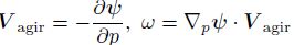
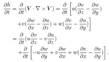
3.1 Helicity and its tendency equationHelicity presents the fluid rotating and moving in the direction of rotation. It is first used to study the turbulence and has the conservation features in the isentropic fluids(Moffatt, 1969, 1981). It is defined as $H=\int \int \int V\cdot \left( \nabla \times V \right)\text{d}\tau $ ; however, the usually used helicity is the local helicity h, and it is defined as
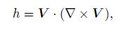
|
(6) |
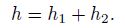
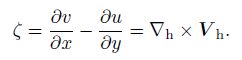
where V =(u, v, w)is the threedimensional wind, and ∇ is the threedimensional differential operator. If Vh represents the horizontal wind, w is the vertical velocity, and ζ is the vertical component of the vorticity, the local helicity can be rewritten as
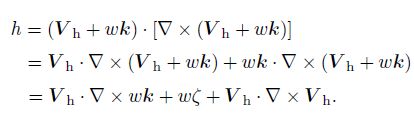
|
(7) |
By further defining V χ and V ψ as the divergent component and rotating component of horizontal wind V h, the horizontal helicity can be rewritten as
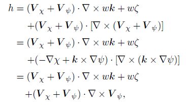
|
(8) |
where χ and ψ present the potential function and the stream function.
It is seen that the helicity is the combined action of the projection of the vortex onto divergent wind, convergent wind, and vertical velocity. For the strong mesoscale system, the divergent wind and the vertical velocity are both strong. Thus, the helicity is a better descriptor. The sign of the helicity indicates the com bination of the vorticity and the velocity. Helicity has first been used to study the storms with strong convections by Lilly(1986a, b). Then, it has been used in the numerical simulations and the observation analysis of storms(Brooks et al., 1993; Davies and Johns, 1993; Johns et al., 1993). Wu and Tan(1989)deduced the helicity equation and pointed out that when the friction is neglected, the helicity is conserved in the quasigeostrophic motions. Besides, Wu et al.(1992) and Liu and Liu(1997)discussed the application of the helicity to the maintenance of the storms and the weather analysis of strong convection.
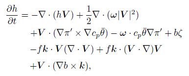
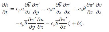
According to Lu and Gao(2003), in the adiabatic, frictionless, and local rectangular coordinate system, the helicity equation can be written as
|
(9) |
where b = gθ'/θ; g is the acceleration of gravity; θ' is the perturbation of potential temperature;
θ = θ(z)is the basic state of potential temperature; ω = ∇ × V =(ω1, ω2, ζ)is the relative vorticity, and 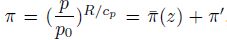
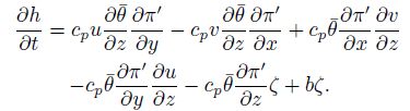
According to Lu and Gao(2003)(also see the Appendix), Eq.(9)can be simplified by ignoring the terms smaller than the buoyancy term and be written as
|
(10) |
In the vector form, it is
|
(11) |
Besides, there is
|
(12) |
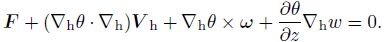
According to Lu and Gao(2003), the local varia tion term of the helicity is in the same magnitude with the advection term of the helicity, and they are both the small terms in the equation. Besides, the first five terms on the right hand side of Eq.(10)are larger than the sixth term. Just keep the bigger terms in the equation and we can obtain the following balance equation
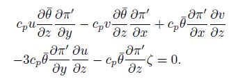
|
(13) |
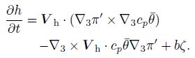
In the vector form,
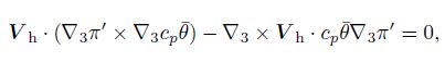
|
(14) |
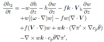
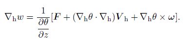
where the subscript “h” indicates horizontal, the sub script “3” indicates that partial derivation is calcu lated in all the three directions. If the vertical velocity has been partly retained in the balance equation, Eq. (14) can be simplified into
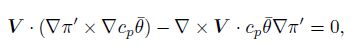
|
(15) |
where V is the threedimensional wind. Laplace operator ∇ is also three dimensional.
Equations(14)and(15)both include divergent winds. Further present V as V = V h + wk, V h = V ψ + V χ, then Eqs.(14)and(15)become
|
(16) |
|
(17) |
It is seen that the balance equations deduced from he licity include the divergent wind and rotational wind, thus they can better describe the interactions between the two types of winds. From Eq.(16), since there is vertical velocity, the balance equation can reflect the interactions among the divergent wind, rotational wind, and vertical motion in the dynamic balance systems. Moreover, as the rotational wind has two terms, it is the main factor in the equations. This is the general features of balance. Thus, we take Eqs.(14)and (15) as the mesoscale balance equations.
3.3 Mesoscale imbalance equationIn Section 3.2, we have obtained the mesoscale balance Eqs.(14)and(15). Then, we will discuss the variation of helicity when the balance equations have been destroyed.
When it is in imbalance, there is

|
(18) |
where O(ε)is the difference between the two terms in the left side of the equation. Now the helicity equation can be written as
|
(19) |
If we classify the imbalance process into two steps, i.e., the destruction and the reconstruction steps, we can obtain the imbalance equations respectively for the two steps by the decomposition analysis method proposed by Chen(1987)as follows.
|
(20) |
|
(21) |
|
(22) |
Equation(20)represents the impact of the balance destruction due to the horizontal advection and the horizontal convergence and divergence on the local variation of helicity. Equation(21)represents the variations of the helicity caused by the adjustment of the imbalance to the balance by the vertical motions due to the destruction of balance. Here we take Eq. (19)as one of the mesoscale imbalance equations, and Eq.(19)can be used to diagnose the mesoscale imbalance flow.
Besides, we can also use the divergence equation as the mesoscale imbalance equation. It is another kind of mesoscale imbalance equation.
The horizontal divergence equation is
|
(23) |
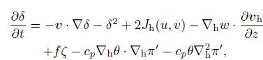
where δ is the horizontal divergence. Generally, the square of the divergence is smaller than the others, so Eq.(23)can be further simplified as

|
(24) |
By calculating the terms on the righthand side of Eq.(24), we can know the variation of the divergence and the intensity of the imbalance. Moore and Abeling(1988)used divergence equation to diagnose the imbalance. Meanwhile, by combing the continuity equation, we can know the vertical motions during the imbalance process.
Since the mesoscale motion can be considered as ∂θ
field.
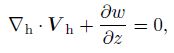
uncompressible, there is 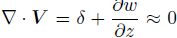
|
(25) |
If the variation of horizontal divergence is known, we can determine the variations of the vertical motions with height.
Equation (24) has taken the baroclinic effect of the atmosphere into consideration. Moreover, if the thermal dynamic force has also been considered, from the adiabatic thermal dynamic equation, there is
|
(26) |
where θ is potential temperature. Apply the differential operator ∇h to Eq. (26), we obtain
|
(27) |
Furthermore, there is
|
(28) |
Because ∇h × ∇hθ = 0, the above equation can be simplified as
|
(29) |
and
|
(30) |
Then, we have
|
(31) |
Denoting 
|
(32) |
From Eq. (32), it is seen that different $\frac{\partial \theta }{\partial z}$ would af fect the actions of the thermal dynamic field. When $\frac{\partial \theta }{\partial z}=0$ , the atmosphere is neutral stratification, thus there is no force on the air particle, and there is no impact of θ on the vertical motion w. From Eq. (25), the horizontal divergence will not be affected by θ, and it is mainly affected by the dynamical field. However, the condition of $\frac{\partial \theta }{\partial z}=0$ is hard to widely obtain in reality; for most cases, $\frac{\partial \theta }{\partial z}\ne 0$.
When $\frac{\partial \theta }{\partial z}\ne 0$, from Eq. (32), we can obtain
|
(33) |
Then, there is
|
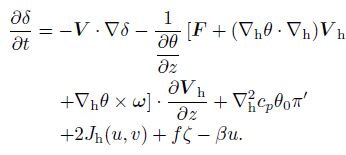
(34) |
Equation(34)is the imbalance equation that contains the baroclinic effect and the thermal dynamical forcing on the adiabatic, frictionless, and nonneutral stratification conditions. It is also called the divergence tendency equation.
4 Mesoscale balance models and their related PV inversionIn the above section, we have introduced the mesoscale balance equations. In this section, we will introduce the mesoscale balance models constructed based on the above balance equations and the cor responding PV inversion. The PV inversion means that we can deduce the other dynamical fields such as wind, temperature, pressure, etc. by the PV on the isentropic surface. Its precondition is that there is balance, and there is no gravity wave or inertial grav ity wave. It is seen that the PV inversion is closely connected to the balance models. Thus, we will first introduce the balance models then the PV inversion.
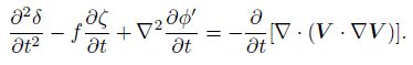
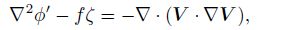
4.1 Mesoscale barotropical balance models and the PV inversionNeglecting the time tendency term in the diver gence equation, McIntyre and Norton(2000)estab- lished the mesoscale balance models as following
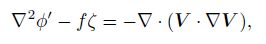
|
(35) |
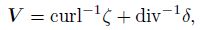
where φ' is the departure of the geopotential φ from a constant reference value φ, and the wind is defined as
|
(36) |
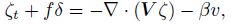
The vorticity, divergence, and continuity equa tions can be obtained by the barotropic shallow equa tions, and they can be written as
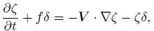
|
(37) |
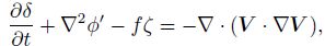
|
(38) |
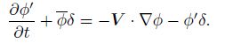
|
(39) |
The derivation of Eq. (38) is
|
(40) |
From Eqs. (37), (39), and (40), we can further obtain
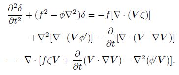
|
(41) |
Supposing 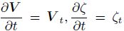
|
(42) |
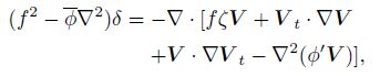
|
(43) |
|
(44) |
|
(45) |
|
(46) |
|
(47) |

|
(48) |
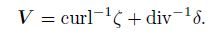
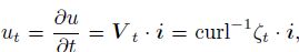
Taking the PV conservation $\frac{\text{d}Q}{\text{d}t}=0$ as forecast equation, we have $\frac{\partial Q}{\partial t}=-V\cdot \nabla Q$. If we know the wind and the PV at time n, we can deduce the PV at time n+1 by the integration. Thus, Qn+1 is a known quantity. Then, Eqs. (42)-(47) form a set of closed equations that have six unknown quantities, and we can solve these equations to obtain the unknown quan tities $\left( \phi \prime ,V,\varsigma ,\delta ,{{V}_{t}},{{\varsigma }_{t}} \right)$. Further, by solving Eq. (48), we can obtain the flows at different times. Since the di vergent wind has been contained in the model (formed by Eqs. (42)-(48)), and the model has been obtained based on the large-scale barotropical models, we call the model the mesoscale barotropical balance models. McIntyre and Norton (2000) had called the largescale barotropical balance model as the first class balance model, and the above balance model as the second class balance model. Similarly, we can deduce the third class balance model by further differentiating Eqs. (40) and (37), and take V t = curl-1ζt +div-1δt, and ${{V}_{2}}=\frac{{{\partial }^{2}}V}{\partial {{t}^{2}}}=\text{cur}{{\text{l}}^{-1}}{{\varsigma }_{2}}$, combined with vortic- ity equation and PV conservation equation, etc. to form the closed equations. We can similarly obtain the fourth class balance model, fifth class balance model, and so on. It is seen that the higher the class, the more important the divergent wind, and the more suitable the model is for the mesoscale system.
4.2 Mesoscale baroclinical balance models and the PV inversionThe mesoscale baroclinical balance models are es tablished based on the mesoscale balance Eq. (15),combined with the PV conservation, potential temper ature conservation, expressions of the absolute vortic ity, PV, π, etc.

|
(49) |
|
(50) |
|
(51) |
|
(52) |

|
(53) |

|
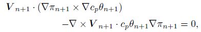
(54) |
It seems that it is a closed equation set. However, because V is vector, it can be separated into three components, thus the equation set has two more un known quantities, and the equation set is not closed. More appropriate equations should be added. Here, we further consider the divergence equation
|
(55) |
Since the time tendency of the divergence has been neglected due to its small magnitude, Eq. (55) is simplified as
|
(56) |
Supposing that the atmosphere is uncompressible in balance condition, there is
|
(57) |
and the vertical vorticity is
|
(58) |
Now Eqs. (49){(58) have made up a closed equa
tion set, and the unknown quantities can be solved
by this equation set now. It is noted that V con
tains both the divergent and rotational winds. In nu
merical calculation, from PV conservation ($\frac{\text{d}Q}{\text{d}t}=0$),
we know
$\frac{\partial Q}{\partial t}=-V\cdot \nabla Q$. In difference format, it is 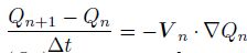
|
(59) |
|
(60) |
|
(61) |
|
(62) |
|
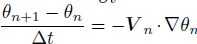
(63) |
|
(64) |
where Qn+1 and θn+1 are known quantities. According to the above euqaitons, we can obtain πn+1, V n+1, ωan+1, and ρn+1 at time n + 1. If the wind and temperature at the initial time are known, we can calculate the corresponding vorticity, potential temperature, and the PV. According to the PV conservation and potential temperature conservation, we can obtain PV and potential temperature at the next time, designated as Qn+1 and θn+1. Then, by using the balance model, π, V, ωa, and ρ at the next time (πn+1, V n+1, ωa n+1, and ρn+1 )will be known as well. Similarly, we can obtain πn+2, V n+2, ωan+2, ρn+2, and so on. Thus, the values of π, V, ωa, and ρ at the future time will be known. Namely, the flows of the balance model will be known.
The above mesoscale barotropical balance model, baroclinical balance model, and their corresponding PV inversion techniques can be used to diagnose the mesoscale imbalance flows. The fields obtained by the PV inversion are the balance fields, and when they are compared with the real fields, the imbalance can be diagnosed.
5 Summary and discussionIn this paper, after reviewing the largescale balance and imbalance equations and a series of tools for diagnosing the imbalance flows, the mathematical definition of the balance equation and imbalance equation have been presented, and their physical meanings are explained; meanwhile, the concept of balance model is proposed.
Considering that there is balance motion in the meososcale weather system, we pointed out that there are balance equations and balance models for describing the mesoscale system, and correspondingly, there are imbalance equations and imbalancediagnosis tools. From the features of mesoscale convective system and mesoscale convective complex, it is seen that the vortex, divergence, and vertical motion play important roles in mesoscale systems. The largescale balance equation has limitations to describe the mesoscale balance motions. We proposed that deduc ing the mesoscale balance equation from the helicity equation since it can contain the rotating wind, divergent wind, and vertical motion simultaneously.
The mesoscale balance and imbalance equations have presented in the local rectangular coordinate system with adiabatic and frictionless assumptions. The combinations of the balance equation with the vorticity equation, the divergence equation, the continuity equation, and the thermaldynamical equation, formed a mesoscale balance model, of which the balance equation is the core. Further, using the PV conservation and the potential temperature conservation, the flows of the mesoscale balance model can be deduced, and their comparison with the real fields gives the degree of the imbalance.
Generally, the proposed mesoscale balance equations and models, and their corresponding PV inversion techniques can be used to diagnose the mesoscale balance and imbalance flows. Their application to the real cases will be given in the next paper.
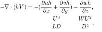
Appendix Scale Analysis on Helicity Equation
Denote U, V, and W as the characteristic scales
level in the equal entropy atmosphere, we define it
of horizontal and vertical winds, Lx, Ly, and D the
characteristic scales of horizontal and vertical lengths
of perturbations, Θ' and Θ the characteristic scales of θ/ and θ, ∆hΘ' the characteristic scales of horizontal variations of θ', while ∆hΘ and ∆z Θ the characteristic scales of horizontal and vertical variations of θ,
∆hΠ and ∆z Π the characteristic scales of horizontal
and vertical variations of π', Ω the characteristic scale of Colioris parameter f, and H the height at the Θ level in the equal entropy atmosphere, we define it as 
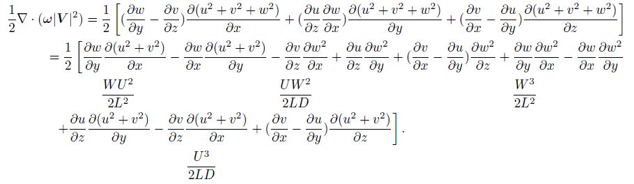
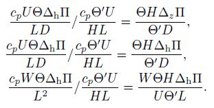
The first term:
|
The second term:
|
The third term:
|
The fourth term:
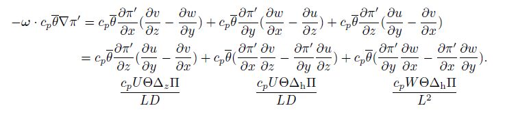
|
The fifth term:
|
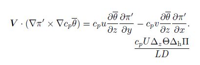
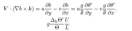
Moreover, there is 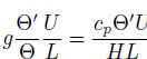
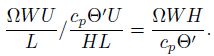
The sixth and the seventh terms are resulted from the coriolis forcing, thus we consider them together:
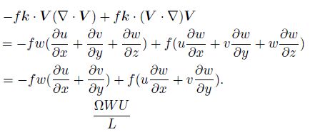
|
The second term:
|
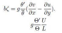
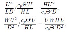
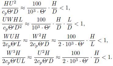
Divide the above terms by the buoyancy term bζ (the fifth term), then we have
The first term:
|
The second term:
|
The third term:
|
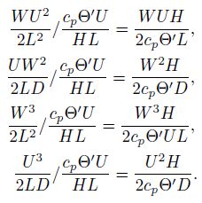
The fourth term:
|
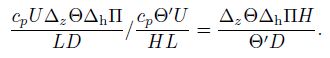
The sixth and seventh terms:
|
The eighth term:
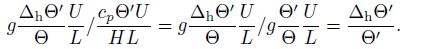
|
As far as the mesoscale motions at the midlatitude are concerned, the magnitudes of the above characteristic scales are as follows.
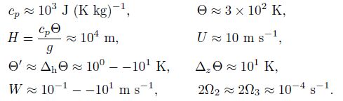
|
For deep convection, $\frac{D}{H}$
is a little smaller than
1, and the vertical motion is strong, namely W ≈ U.
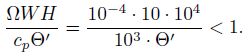
Besides, there are 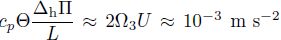
|
It is seen that compared with the buoyancy term, they can be neglected. The third and fourth terms are
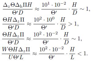
|
The sixth and seventh terms:
|
The eighth term:
|
Keep those comparable or larger than 1 in Eq. (9), then we have
|
| Allen J. S, J. A. Barth, P. A. Newberger. ,1990: On intermediate models for barotropic continental shelf and slope flow elds. Part I:Formulation and comparison of exact solutions. J. Phys. Oceanogr. , 20 , 1017–1043. |
| Barth J. A, J. S. Allen, P. A. Newberger. ,1990: On intermediate models for barotropic continental shelf and slope flow elds. Part Ⅱ:Comparison of numer-ical model solutions in doubly periodic domains. J. Phys. Oceanogr. , 20 , 1044–1076. |
| Brandes E. A. ,1990: Evolution and structure of the 6-7 May 1985 mesoscale convective system and associ-ated vortex. Mon. Wea. Rev. , 118 , 109–127. DOI:10.1175/1520-0493(1990)118<0109:EASOTM>2.0.CO;2 |
| Brooks H. E, C. A. Doswell, R. Davies-Jones. ,1993: Environmental helicity and the maintenance and evolution of low-level mesocyclones. The Tornado:Its Structure, Dynamics, Prediction, Hazards.Church, C., D. Burgess, C. Doswell, et al., Eds., American Geophysical Union , 79 , 97–104. DOI:10.1029/GM079 |
| Cao J, Q Xu. ,2011: Computing hydrostatic poten-tial vorticity in terrain-following coordinates. Mon. Wea. Rev. , 139 , 2955–2961. DOI:10.1175/MWR-D-11-00083.1 |
| Charney J. G. ,1955: The use of the primitive equations of motion in numerical prediction. Tellus , 7 , 22–26. DOI:10.1111/tus.1955.7.issue-1 |
| Charney J. G. ,1962: Integration of the primitive and balance equations. Proc. Int. Symp. Numerical Weather Prediction. Meteor. Soc. Japan, Tokyo , 131 , 131–152. |
| Chen Qiush. ,1987: Dynamics of Synoptic Systems and Subsynoptic Systems , 8–26. |
| Davies J. M, R. H. Johns. ,1993: Some wind and instability parameters associated with strong and violent tornadoes. 1:Wind shear and helicity. The Tornado:Its Structure, Dynamics, Prediction, Hazards. Church, C., D. Burgess, C. Doswell, et al., Eds., American Geophysical Union , 79 , 573–582. |
| Deng Difei, Zhou Yushu. ,2011: Analysis and ap-plication of irrotational wind component in the drastically increasing and decreasing processes of ‘Saomai' typhoon. Plateau Meteor. , 30 , 406–415. |
| Ding Yihui. ,2005: Advanced Synoptic Meteorology. China Meteorological Press, Beijing , 80 . |
| Doswell Ⅲ C. A. ,1987: The distinction between large-scale and mesoscale contribution to severe convec-tion:A case study example. Wea. Forecasting , 2 , 3–16. DOI:10.1175/1520-0434(1987)002<0003:TDBLSA>2.0.CO;2 |
| Fritsch J. M, J. D. Murphy, J. S. Kain. ,1994: Warm core vortex amplication over land. J. Atmos. Sci. , 51 , 1780–1807. DOI:10.1175/1520-0469(1994)051<1780:WCVAOL>2.0.CO;2 |
| Fu Shenming, Sun Jianhua, Zhao Sixiong, et al. ,2011: The energy budget of a southwest vortex with heavy rainfall over South China. Adv. Atmos. Sci. , 28 , 709–724. DOI:10.1007/s00376-010-0026-z |
| Fu S. M, J. P. Zhang, J. H. Sun, et al. ,2015: Compos-ite analysis of long-lived mesoscale vortices over the middle reaches of the Yangtze River valley:Octant features and evolution mechanisms. J. Climate , 29 , 761–781. DOI:10.1175/JCLI-D-15-0175.1 |
| Gao Shouting, Zhou Feifan. ,2006: Mesoscale balance equation and the diagnostic method of unbalanced flow based on helicity. Chinese J. Atmos. Sci. , 30 , 854–862. |
| Holton, J. R., 2004:An Introduction to Dynamic Meteo-rology. 4th Ed., Academic Press, 535 pp. |
| Hoskins B. J, F. P. Bretherton. ,1972: Atmospheric frontogenesis models:Mathematical formulation and solution. J. Atmos. Sci. , 29 , 11–37. DOI:10.1175/1520-0469(1972)029<0011:AFMMFA>2.0.CO;2 |
| Hoskins B. J. ,1975: The geostrophic momentum ap-proximation and the semi-geostrophic equations. J. Atmos. Sci. , 32 , 232–242. |
| Houez R. A. Jr, B. F. Smull, P. Dodge. ,1991: Mesoscale organization of springtime rainstorms in Oklahoma. Mon. Wea. Rev. , 118 , 613–654. |
| Johns R. H, J. M. Davies, P. W. Leftwich. ,1993: Some wind and instability parameters associated with strong and violent tornadoes:2. Variations in the combinations of wind and instability parameters.The Tornado:Its Structure, Dynamics, Prediction, Hazards. Church, C., D. Burgess, C. Doswell, et al., Eds., American Geophysical Union , 79 , 583–590. |
| Keyser D, B. D. Schmidt, D. G. Duffy. ,1989: A technique for representing three-dimensional verti-cal circulations in baroclinic disturbances. Mon. Wea. Rev. , 117 , 2463–2494. DOI:10.1175/1520-0493(1989)117<2463:ATFRTD>2.0.CO;2 |
| Leary C. A, E. N. Rappaport. ,1987: The life cy-cle and internal structure of a mesoscale convective complex. Mon. Wea. Rev. , 115 , 1503–1527. DOI:10.1175/1520-0493(1987)115<1503:TLCAIS>2.0.CO;2 |
| Lilly D. K. ,1986a: The structure, energetics and propa-gation of rotating convective storms. Part I:Energy exchange with the mean flow. J. Atmos. Sci , 43 , 113–125. |
| Lilly D. K. ,1986b: The structure, energetics and prop-agation of rotating convective storms. Part Ⅱ:He-licity and storm stabilization. J. Atmos. Sci , 43 , 126–140. |
| Liu Shikuo, Liu Shida. ,1997: Toroidal-poloidal de-composition and Beltrami flows in atmosphere mo-tions. Chinese J. Atmos. Sci. , 21 , 151–160. |
| Liu Shikuo, Sun Feng. ,2000: Scale analysis and phys-ical mechanism of semi-geostrophic adaptation in the tropical atmosphere. Chinese J. Atmos. Sci. , 24 , 26–40. |
| Lu Huijuan, Gao Shouting. ,2003: On the helicity and the helicity equation. Acta Meteor. Sinica , 61 , 684–691. |
| Lynch P. ,1989: The slow equations. Quart. J. Roy. Meteor. Soc. , 115 , 201–219. DOI:10.1002/(ISSN)1477-870X |
| McIntyre M. E, W. A. Norton. ,2000: Potential vorticity inversion on a hemisphere. J. Atmos. Sci. , 57 , 1214–1235. DOI:10.1175/1520-0469(2000)057<1214:PVIOAH>2.0.CO;2 |
| Moffatt H. K. ,1969: The degree of knottedness of tan-gled vortex lines. J. Fluid Mech. , 35 , 117–129. DOI:10.1017/S0022112069000991 |
| Moffatt H. K. ,1981: Some developments in the theory of turbulence. J. Fluid Mech. , 106 , 27–47. DOI:10.1017/S002211208100150X |
| Moore J. T, W. A. Abeling. ,1988: A diagnosis of unbalanced flow in upper levels during the AVE-SESAME I period. Mon. Wea. Rev. , 116 , 24252436. |
| Raymond D. J. ,1992: Nonlinear balance and potential-vorticity thinking at large Rossby number. Quart. J. Roy. Meteor. Soc. , 118 , 987–1105. DOI:10.1002/(ISSN)1477-870X |
| Wu Rongsheng, Tan Zhemin. ,1989: Conservative laws on generalized vorticity and potential vorticity and their applications. Acta Meteor. Sinica , 47 , 436442. |
| Wu W. S, D. K. Lilly, R. M. Kerr. ,1992: Helicity and thermal convection with shear. J. Atmos. Sci. , 49 , 1800–1809. DOI:10.1175/1520-0469(1992)049<1800:HATCWS>2.0.CO;2 |
| Xu Q. ,1994: Semibalance model-connection between geostrophic-type and balanced-type intermediate models. J. Atmos. Sci. , 51 , 953–970. DOI:10.1175/1520-0469(1994)051<0953:SMBGTA>2.0.CO;2 |
| Zhang Fuqing, S. E. Koch, C. A. Davis, et al. ,2000: A survey of unbalanced flow diagnostics and their application. Adv. Atmos. Sci. , 17 , 165–183. DOI:10.1007/s00376-000-0001-1 |
| Zhang D. L, J. M. Fritsch. ,1988: A numerical inves-tigation of a convectively generated, inertially stable, extratropical warm-core mesovortex over land. Part I:Structure and evolution. Mon. Wea. Rev. , 116 , 2660–2687. |