 2016, Vol. 28
The Chinese Meteorological Society
Article Information
- XIAO Ziniu, LI Delin. 2016.
- Solar Wind: A Possible Factor Driving the Interannual Sea Surface Temperature Tripolar Mode over North
- J. Meteor. Res., 28(3): 312-327
- http://dx.doi.org/10.1007/s13351-016-5087-1
Article History
- Received October 12, 2015;
- in final form March 3, 2016


2 State Key Laboratory of Numerical Modeling for Atmospheric Sciences and Geophysical Fluid Dynamics, Institute of Atmospheric Physics, Chinese Academy of Sciences, Beijing 100029
The dominant mode of interannual variation in wintertime North Atlantic sea surface temperature(SST)is observed as a meridional tripolar anomaly pattern that spans the basin,with a colder subpolar region,a warmer midlatitude region,and a colder region between the equator and 30°N(Sutton et al., 2000; Czaja and Marshall, 2001; Marshall et al., 2001; Wu and Liu, 2005; Fan and Schneider, 2012). Because of its importance both as an external forcing and a relatively reliable climatic predictor,the North Atlantic SST tripole ties closely to the variations of weather and climate in certain continents. In particular,Rodríguez-Fonseca et al.(2006)suggested that persistence of the summer subtropical SST signal in one part of the North Atlantic SST tripole could be helpful in predicting the upcoming winter precipitation pattern over Europe and North Africa. Wu et al.(2010)showed that the SST tripolar pattern in the preceding spring is partly responsible for the interannual variations in summer temperature in Northeast China,when the relationship between ENSO and Northeast China summer temperature is weak. With numerical models,Sutton et al.(2000)demonstrated that the significant positive temperature anomalies over east ern North America appear to be due to the SST tripolar pattern. Furthermore,Li et al.(2003)reported the asymmetric impacts of the North Atlantic SST tripole on rainfall in Northwest Africa in early–mid and late winter,based on a large ensemble of general circulation model simulations.
Numerous studies have uncovered the inseparable connection and strong dependence between the wintertime SST tripolar pattern and the North Atlantic Oscillation(NAO),characterized by a prominent large-scale oscillation in sea level pressure(SLP)between the Icelandic low and the Azores high(Delworth,1996; Czaja and Frankignoul, 1999; Marshall et al., 2001; Hurrell et al., 2003; Wang et al., 2004; Cassou et al., 2007). Therefore,the North Atlantic SST tripole and the NAO could be unified to some extent into one coupled ocean–atmosphere phenomenon during boreal winter. An understanding of the mechanisms of this phenomenon will help us better predict climate variability in North Atlantic and other remote areas. Among the various mechanisms proposed,the influence of solar activity has drawn increasing attention in recent years(Bond et al., 2001; Shindell et al., 2001; Boberg and Lundstedt, 2002,2003; Kodera and Kuroda, 2005; Ineson et al., 2011; Li et al., 2011; Scaife et al., 2013).
A large amount of observational evidence has indicated that the changes in the North Atlantic climate are partly influenced by solar activity. Statistical studies have shown that the intensity,spatial structure,and center position of the NAO during boreal winter differ significantly in different phases of the 11-yr solar cycle(Kodera, 2002,2003; Kodera and Kuroda, 2005; Huth et al., 2006; Maliniemi et al., 2014). Using an idealized coupled climate model,Scaife et al.(2013)displayed that both the NAO and the SST tripolar pattern in North Atlantic appear to lag a few years behind the changes in solar ultraviolet radiation levels. Lu et al.(2008)found that the solar wind(SW)dynamical pressure is closely associated with the Northern Annular Mode,which could represent the surface NAO behavior. Zhou et al.(2014)explored contemporaneous correlations between the winter NAO index and different proxies of solar activity during 1963– 2011,such as the sunspot number(SSN),10.7-cm solar radio flux(F10.7 cm),solar wind speed(SWS),and the SW geoeffective electric field defined by Boberg and Lundstedt(2002). They pointed out that unlike other solar parameters,the SWS is strongly correlated with the NAO. Thus,the SW could be considered as a causal mechanism influencing the formation of the NAO.
As a measure of solar activity,the SW resembles the high speed stream generated from solar coronal holes. This stream,which mainly consists of electrons,protons,and Alpha particles with energies,varies in density,temperature,and speed over time. Other aspects of solar activity,such as the SSN,F10.7 cm,and total solar irradiance,which vary with the 11-yr cycle,are broadly used to characterize the intensity of solar irradiation. The SW can violently interact with the earth’s magnetosphere,causing associated energetic particle precipitation(EPP)to descend into the earth’s upper and mid atmosphere at high geomagnetic latitudes(Clilverd et al., 2006). Then,the nitrogen oxides(NOx)enhancement caused by EPP can lead indirectly to polar stratospheric ozone loss and slow alterations of dynamical and thermal conditions of the stratosphere via certain chemical process(Solomon et al., 1982; Randall et al., 2005,2007; Baumgaertner et al., 2011; Seppälä et al., 2013). On the other hand,Boberg and Lundstedt(2002) suggested that the downward propagation of SW-induced electromagnetic disturbance might represent a dynamic process by which the SW signal can penetrate into the lower troposphere. Recently,Tinsley(2008,2012)and Mironova et al.(2012)suggested a much more direct and rapid forcing process of SW on the stratosphere and troposphere. Because of the existence of geomagnetic field,SW particles cannot penetrate directly into the mid and lower atmosphere; however,the electromagnetic disturbance generated by the SW particles in the global atmospheric electric circuit can rapidly extend into the lower atmosphere in the subauroral zone,where they can influence the cloud cover,and consequently alter the atmospheric conditions in the troposphere through cloud microphysics process.
The question is raised,therefore,of whether the SW is a key factor driving the earth’s climate. Motivated by the research above,the present study attempts to answer the following questions:(1)Are the variations in the SWS highly connected to the North Atlantic SST tripolar mode and its overlying atmospheric circulation? (2) Is the magnitude of SWS critical in creating the SST tripole in the North Atlantic sector? (3) How does it work? To this end,here we explore the effects of SW on interannual variability in the North Atlantic SST during boreal winter through analysis of observational data. Furthermore,we discuss the relevant processes and possible mechanisms whereby the SW may influence the interannual North Atlantic SST variability,by identifying the changes in atmospheric circulation,air temperature,and cloud cover,acting in concert with SWS variations.
2. Data and methodsWe employ the daily SWS data obtained from the OMNI database of the Goddard Space Flight Center of NASA(ftp://spdf.gsfc.nasa.gov/)(King and Papitashvili, 2005)as a measure of SW intensity. These SWS data are available from December 1963 onward. Other measure of the intensity of solar activity,such as the SSN,is provided by the NOAA(http://www.ngdc.noaa.gov/). We use the monthly gridded SST analysis based on the NOAA Extended Reconstructed SST version 3(ERSST V3)product(Xue et al., 2003; Smith et al., 2008)from December 1963 to February 2013(selected to match the time range of the available SWS data). The monthly gridded data of SLP,zonal wind,and air temperature are taken from the NCEP/NCAR reanalysis dataset(Kalnay et al., 1996),also for the same period. The cloud cover data are obtained from the International Comprehensive Ocean–Atmosphere Dataset(ICOADS)of the NOAA(Woodruff et al., 2005,2011). In this paper,winter is designated as the consecutive months of December,January,and February(DJF). All data are averaged into wintertime means. The linear trends of these wintertime gridded data are removed before analysis.
The dominant interannual mode of the North Atlantic SST in winter is defined by an empirical orthogonal function(EOF)analysis. To characterize the period of SWS variations and the leading EOF time series of SST in North Atlantic,a power spectrum analysis is applied. Furthermore,a linear regression analysis between SWS and North Atlantic SST is used to identify the SST anomaly(SSTA)pattern that accompanies the SWS variations. A composite mean difference method is used to examine the impacts of SW on the North Atlantic SST and its overlying atmospheric circulation and cloud cover,for typical high and low SWS years selected from the study period.
3. Results 3.1 Relationship between SST and SWSPrevious analyses have demonstrated the close association between the NAO and SWS,not only on the day-to-day timescale but also on the year-to-year timescale(Zhou et al., 2014). How do the SSTs vary with respect to SWS variations over the entire North Atlantic Ocean and other basins? The global correlation maps between SWS,SSN,and SST in wintertime(Fig. 1)show areas where the SST increases and decreases significantly with the acceleration of SWS(Fig. 1a),such as in North Atlantic,high-latitude South Atlantic,and the tropical and midlatitude Indian Ocean regions. However,only a few scattered areas related significantly and positively with SSN appear in North Pacific,South Atlantic,and the South Indian Ocean regions(Fig. 1b). This paper focuses on the relationship of SW and SSTA in North Atlantic,so the signal in the Indian Ocean is not discussed here. In the two correlation maps of Fig. 1,SWS shows a close relationship with the SST over North Atlantic. Distribution of their correlation coefficients in the North Atlantic region demonstrates a sandwich pattern(Fig. 1a),with positive correlations in midlatitudes and negative correlations over low-and high-latitudes,broadly similar to the pattern of SST tripolar mode.
 |
| Fig. 1. Correlation maps between DJF-mean SST and DJF-mean (a) SWS and (b) SSN. Areas with the 95% confidence level are indicated by black dots. |
To detect the relationship between SWS variations and the change in the North Atlantic SST during boreal winter,features of the North Atlantic SST variability are analyzed. We first extract the primary EOF mode of wintertime interannual SST variability over North Atlantic(5°–75°N,100°W–15°E)during 1964–2013(Fig. 2). Figure 2a shows the spatial pattern of the first EOF mode of the North Atlantic SST(hereafter referred to as SST EOF1),which accounts for 27.7% of the total variance,11.2% more than the second EOF mode. The SST EOF1 exhibits a positive meridional tripolar pattern spanning the entire North Atlantic basin,with a colder subpolar region,a warmer midlatitude region,and a colder low-latitude region. This SST tripolar mode,which has centers near the northeast of Newfoundland,along the southeast coast of the United States,and along the west coast of North Africa,is very similar to the high-correlation pattern between the SWS and SST over the North Atlantic shown in Fig. 1a. In addition,the corresponding time series of SST EOF1(Fig. 2b)exhibits pronounced characteristics of interannual and interdecadal fluctuations.
 |
| Fig. 2. (a) Spatial pattern of the first EOF mode (EOF1) of observed DJF-mean SST in the North Atlantic region (5°–75°N, 100°W–15°E). This mode explains 27.7% of the total variance, 11.2% more than the second EOF mode. (b) Standardized time series of SST EOF1. |
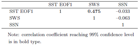
To examine the SW impacts on the SST EOF1,we calculate the contemporaneous correlations between the time series of SST EOF1 and different solar activity parameters,including winter-mean SWS and SSN from 1964 to 2013(Table 1). The SWS is strongly correlated with SST EOF1(r = 0.475,at the 99% confidence level). To consider autocorrelations between the interdecadal evolution of SWS and SST EOF1,the effective degrees of freedom is calculated based on Davis(1976)and Chen(1982). The effective number of degrees of freedom is 37,which is a stricter criterion than that used earlier. In addition,the correlation between SWS and SST EOF1(0.475)is still significant at the 99% confidence level(0.408). However,no significant correlations can be found for SST EOF1 and SSN. Therefore,it is SWS rather than SSN that plays an important role in the solar influence on North Atlantic climate during concurrent winter.
 |
A period analysis is employed to detect the similarities in variations of SWS and the North Atlantic SST tripolar mode. Time series of standardized DJFmean SST EOF1,SWS,and SSN are plotted in Figs. 3a–c,for the period 1964–2013,respectively. The temporal trends show that the SWS is subject to more variability than the SSN,which is more similar to the time series of SST EOF1. As shown in Fig. 3e,the SWS has characteristic variations on multiple timescales,especially at 11-yr cycle like the SSN. The black dashed line superimposed on the data in Fig. 3b represents a 5-point smoothing curve,which indicates that the SWS peaks typically occur in the descending phase 2–5 yr after the maximum SSN. Moreover,the power spectra for SST EOF1 in Fig. 3d and for SWS in Fig. 3e are analogous,and both demonstrate an obviously around 4-yr periodicity that does not appear in Fig. 3f for the SSN. McIntosh et al.(2015)inferred that the annual variations in the SWS are likely driven by changes in the bands of strong magnetic fields in each solar hemisphere. The similarity between the period spectra of SWS and SST EOF1 implies a possible intrinsic linkage between the SWS and the North Atlantic SST tripolar mode.
 |
| Fig. 3. (a, b, c) Time series and (d, e, f) power spectrum of standardized wintertime (a, d) DJF-mean SST EOF1, (b, e) SWS, and (c, f) SSN for the period 1964–2013. The black dashed line in (b) superimposed on the time series of SWS denotes a five-point smoothing curve. |
Do the variations in SWS result in the North Atlantic SST tripolar mode? In this section,we use regression and composite analyses to examine the impacts of interannual variations in SWS on the North Atlantic SST. Owing to the sensitivity of Atlantic Ocean to global climate change(Paeth et al., 1999; Wang and Dong, 2010; Holland and Bruyére,2014),the SST(atmosphere)response to some climate indexes is expected to show a tripole-like(NAO-like)pattern. Thus,we calculate the explained variance for a restricted region(5°–75°N,100°W–15°E)when the SST field is regressed on the standardized SWS,in order to obtain the quantitative contribution of SWS variations to the SST interannual viability in North Atlantic. As shown in Fig. 4,the regressed SST field exhibits warm anomalies off the east coast of the United States and cold anomalies in the subpolar and tropical parts of the North Atlantic Ocean. The regressed SSTA pattern explains 26.6% of the total SST variance in the North Atlantic region and clearly conforms to the documented SST tripolar mode shown in Fig. 2a. In particular,the correlation coefficient be tween the regressed SSTA pattern and SST EOF1 is 0.92,indicating that the SSTA induced by SWS variations could explain most of the variance of the intrinsic interannual SST variability in the North Atlantic region.
 |
| Fig. 4. Distribution of the regression coefficient between the DJF-mean SST and the standardized DJF-mean SWS. This regression pattern accounts for 26.6% of the total variance in North Atlantic (5°–75°N, 100°W–15°E) SST. Black dots indicate the areas with correlation values significant at the 95% confidence level. |
In order to validate the relationship between the SWS and the North Atlantic SST tripolar mode,a composite analysis is conducted to capture the anomalous SST response in North Atlantic to the interannual variations in SWS. The solid/hollow circles in Fig. 5 indicate the typical high/low SWS winters,defined according to the standardized DJF-mean SWS time series,with ±0.8 standard deviation as thresholds. Typical high and low SWS winters are selected,as listed in Table 2. Figures 6a and 6b respectively show the composite SSTA in North Atlantic during typical high and low SWS winters. During typical high SWS winters,SSTA in the North Atlantic basin projects positively onto the SST tripolar mode(Fig. 6a),with warm anomalies over the midlatitudes and cold anomalies to the northeast of Newfoundland and in the lower latitudes. Areas of significance mainly appear in the low-latitude regions(Fig. 6a). Meanwhile,the distribution of SSTA during typical low SWS winters(Fig. 6b)is nearly opposite to that in Fig. 6a. Only some scattered areas in the three centers of SST tripole reaches the 90% confidence level(Fig. 6b). The difference between the SSTs in typical high and low SWS winters over North Atlantic shows a more evident SST tripole(Fig. 6c). The composite analysis above suggests that SWS is very likely the factor driving the North Atlantic SST tripolar mode.
 |
| Fig. 5. The standardized DJF-mean SWS during 1964– 2013. Solid and hollow circles indicate the typical high and low SWS years, respectively. Dashed grey lines represent the threshold values of ±0.8 standard deviation. |

 |
| Fig. 6. (a) Composite SSTA in the North Atlantic region for (a) high SWS winters and (b) low SWS winters. (c) Composite mean difference between the SSTs (℃) in typical high and low SWS winters. Dotted areas indicate significant values at the 90% confidence level. |
How does the SW exert influence on SST and create the North Atlantic SST tripole? Many studies have noted the strong inherent connection between the North Atlantic SST tripole and the atmospheric NAO pattern. Here we consider the atmosphere and ocean surface as an integrated system and examine the circumstances under which a tripolar pattern develops in response to SWS variations.
Linking the SLP distribution with the documented prominent North Atlantic SST tripolar mode(SST EOF1),a positive NAO-like structure is obtained from calculating the correlation coefficient between the time series of SST EOF1 and the winter-mean SLP field(Fig. 7a). The correlation map between SLP and SWS is shown in Fig. 7b. It is clear that a statistically significant strengthening of the Azores high and a de epening of the Iceland low are induced by the increase in the SWS during winter. Although the SLP correlation with the SWS seen in Fig. 7b is weaker than that with SST EOF1 in Fig. 7a,the spatial patterns of the correlations over 10°–85°N,100°W–15°E are correlated with a coefficient of 0.93. Hence,the variation in SWS is highly associated with the North Atlantic SST and the corresponding atmospheric SLP,and the SW is therefore a possible factor influencing both oceanic and atmospheric variability over the North Atlantic region.
 |
| Fig. 7. Correlation maps between the DJF-mean SLP and time series of (a) SST EOF1 and (b) DJF-mean SWS. Dotted areas indicate the 95% confidence level or above. |
Zonal wind plays an essential role in the ocean– atmosphere interactions. To assess the association between the documented mode of the North Atlantic SST tripole and the overlying atmosphere,correlations of zonal-mean zonal wind over North Atlantic(100°W–15°E)with SST EOF1 and SWS are computed separately. The distribution of the correlation coefficients between SST EOF1 and the zonal wind,from sea level up to the stratosphere,is shown in Fig. 8a. The equivalent barotropic tripolar structure of the mean zonal wind is evident in the whole troposphere overlying North Atlantic(Fig. 8a),with positive coefficients occurring at midlatitudes and negative ones at low and high latitudes. A similar pattern is observed for the correlation between the SWS and the zonal-mean zonal wind(Fig. 8b). The significant areas of tripolar structure in both Figs. 8a and 8b extend through the whole troposphere,and even higher into the stratosphere in Fig. 8b. The significant correlations in the high-latitude stratosphere shown in Fig. 8b suggest that the SW signal may be derived from the upper atmosphere. The correlation coefficient of the spatial pattern between Figs. 8a and 8b is greater than 0.93,which further emphasizes that the North Atlantic SST tripolar pattern,as well as the atmospheric circulation tripolar structure,could be governed mainly by the magnitude of SWS.
 |
| Fig. 8. As in Fig. 7, but for the DJF-mean zonal-mean (100°W–15°E) zonal wind rather than the DJF-mean SLP |
As in Section 3.2 for the SSTA,an altitudelatitude cross-section of zonal-mean zonal wind anomalies is shown in Fig. 9. The meridional tripolar patterns present almost completely opposite phases in typical high and low SWS winters(Figs. 9a and 9b). The anomalous intense westerlies appear near the location of the wintertime polar night jet(PNJ)in the stratosphere,and extend to the lower tropo-sphere and the ocean surface during typical high SWS winters(Fig. 9a),in contrast to the weakened westerlies that occur during typical low SWS winters(Fig. 9b). To the north and south of the mentioned westerly anomalies,the westerlies are weakened in high SWS winters,but enhanced in low SWS winters. The difference in composite zonal wind anomalies between the typical high and low SWS winters is shown in Fig. 9c,which reveals a clear vertical meridional tripolar structure with easterly and westerly anomalies. The significant westerly anomalies,accelerated by up to 8 m s−1,are roughly located within 45°–70°N in the whole troposphere and lower stratosphere,while the easterly anomalies appear mainly within 20°–40°N and in high latitudes near the North Pole.
 |
| Fig. 9. As in Fig. 6, but for the DJF-mean zonal-mean (100°W–15°E) zonal wind (m s−1) rather than the SST. |
Boberg and Lundstedt(2002)suggested that the dynamic coupling between the stratosphere and troposphere could provide an explanation for their observations regarding the regional response to the SW variation on winter-to-winter timescales. When the lower stratospheric PNJ is developing and stable,the highlatitude westerlies of the troposphere become stronger than usual(Kuroda and Kodera, 2002; Wallace and Thompson, 2002). In addition,the downward propagation of the signal of abnormal stratospheric zonal mean flow is especially pronounced during the cold season(Baldwin and Dunkerton, 2001). Thus,we examine the climatological monthly mean zonal-mean(100°W–15°E)zonal wind during the cold season from November to March(Figs.10a–e)and the correlation coefficients between DJF-mean SWS and the monthly mean zonal wind(Figs.10f–j). In Figs. 10f–j,we can find that the weak vertical tripolar structure of zonal wind related to the SWS first appears in November. With the downward development and enhancement of PNJ in response to strong radiative cooling over the polar night region from November to January(Figs. 10a–c),the SW-related westerly anomalies become much more evident in the stratosphere and troposphere,with the easterly anomalies lying at the higher and lower latitudes in December. Then,in January,the quasi-barotropic tripolar structure descends into the troposphere and projects significantly onto the positive NAO-like pattern. However,during the weakening period of PNJ,from January to March(Figs. 10c–e),the correlations between SWS and zonal wind also weaken,and in February,the area of significant anomalies is confined only to the high-latitude stratosphere. In March,the correlation pattern changes and inclines poleward. These results highlight the importance of changes in the stratospheric circulation in governing the patterns of wind anomalies of troposphere. More specifically,the acceleration and persistence of PNJ in early winter could promote the extension of the SW signal from the lower stratosphere to the troposphere,while the weakened PNJ in late winter could retard the downward extent of SW signal,and restrict it to the stratosphere. Therefore,the strong dynamic process of stratosphere–troposphere interaction(intensified PNJ)during winter could help the downward penetration of the SW signal into the lower troposphere.
 |
| Fig. 10. (a–e) Climatological monthly mean zonal-mean (100°W–15°E) zonal wind (m s−1) during the cold season (November–March) for the period 1964–2013. (f–j) Correlation coefficients between DJF-mean SWS and monthly mean zonal-mean (100°W–15°E) zonal wind from November to March. Dotted areas indicate statistical significance at the 95% confidence level. |
As we know,the intensity of PNJ is considerably modulated by the meridional temperature gradient in the stratosphere. Previous studies have revealed that the changes in the SW can chemically alter the temperature structure of the stratosphere,and that temperature anomalies appearing as a cooling of the polar upper stratosphere may be a radiative response to the ozone reduction induced by the EPP–NOx(Lu et al., 2008; Baumgaertner et al., 2011; Seppälä et al., 2013). The possibility that the zonal wind anomaly pattern(Fig. 8b)and the strengthened PNJ(Fig. 9a)above are influenced in part by the stratospheric meridional temperature gradient induced by the SW chemical actions is being investigated here in this paper. When taking Fig. 8a into consideration,we notice that the effects of North Atlantic SST tripolar mode(SST EOF1)on the zonal wind can extend into the lower stratosphere. To avoid the impacts of SST tripole on the lower stratosphere,we pay special attention to air temperature at 10,20,and 30 hPa. As displayed in Figs. 11a–c,the climatological winter-mean air temperature in North Pole is colder than that in the mid and low latitudes,indicating that the meridional temperature gradient in the stratosphere can support the development of PNJ in boreal winter. The corresponding global correlation maps between the DJF-mean SWS and air temperature at 10,20,and 30 hPa are displayed in Figs. 11d–f. The common features are a colder polar region and a warmer low-latitude region; specifically,the appearance of significant negative correlations at North Pole and over high-latitude Eurasia,and significant positive correlations in the tropics and over the Gulf of Alaska. These anomalous temperature patterns can generally augment the stratospheric meridional temperature gradient,which indirectly enhances the acceleration and downward development of PNJ,and consequently helps the downward expansion of SW signal. Therefore,the zonal wind anomalies described above could be the indirect result of the greater stratospheric meridional temperature gradient triggered by the chemical effects of higher-speed SW.
 |
| Fig. 11. (a–c) Climatological DJF-mean air temperature (℃) at 10, 20, and 30 hPa for the period 1964–2013. (d–f) Correlation maps between DJF-mean SWS and DJF-mean air temperature at the corresponding levels. Dotted areas indicate statistical significance at the 90% confidence level. |
As described above,the substantial changes in the zonal-mean zonal wind over the North Atlantic Ocean are associated with the interannual variations in SWS. However,it is unclear whether this feature appears only in North Atlantic or exists throughout the entire Northern Hemisphere. With the question in mind,we investigate the global meridional-mean zonal wind and the difference of the zonal wind over 45°–70°N between typical high and low SWS winters(Fig. 12). Enhanced westerly anomalies appear in the stratosphere below 10 hPa. The most striking feature is the pronounced strengthening of the westerlies in the whole troposphere over the North Atlantic Ocean,seeming like a special perforation from the stratosphere to the troposphere. However,the preference of the SW signal for the North Atlantic in particular is not clear. It is possible that an electromagnetic disturbance generated by SW particles in the global atmospheric electric circuit influences electrically the North Atlantic largescale pressure system via cloud microphysics(Tinsley, 2008,2012). Because of the modulation of geomagnetic field,SW particles cannot directly penetrate into the middle and lower atmosphere,but the high energy electrons generated by the SW in the earth’s radiation belt can penetrate into the upper– mid stratosphere over the subauroral zone,where they can change the degree of atmospheric ionization. In addition,the X-ray stimulated by the high-energy electrons can rapidly influence the ionization degree in the lower stratosphere,and even the tropopause over the subauroral zone. In this case,this variation in the ionization degree would substantially alter the global atmospheric electric circuit,and consequently change the atmospheric conditions in the troposphere through cloud microphysics process(Mironova et al., 2012; Tinsley,2012; Huang et al., 2013). This hypothesis is supported by two lines of evidence: the close correspondence between the longitude and latitude of the subauroral zone and those of the Iceland,which is advantageous for high-energy electrons precipitation; and the presence of the semi-permanent Iceland low pressure system,which provides more opportunities for cloud system to develop,and hence avails the development of the cloud microphysics process.
 |
| Fig. 12. As in Fig. 6c, but for the DJF-mean meridionalmean (45°–70°N) zonal wind (m s−1). |
To simply verify this hypothesis,we utilize the cloud cover data to obtain wintertime climatology and composite mean difference of cloud cover between typical high and low SWS winters. As shown in Fig. 13a,the maxima of climatological cloudiness in boreal winter occur in the mid–high latitudes of North Atlantic and North Pacific,mainifesting the locations of the Iceland and Aleutian lows. Notably,the positive anomalies of cloud cover significant at the 90% confidence level occupy the region(45°–65°N)around the Iceland in North Atlantic(Fig. 13b). The features in Fig. 13b further confirm that,as compared with the location of the Aleutian low,the Iceland low is much closer to the subauroral zone,where there might be an important and peculiar entry to earth for the SW. Thus,the analyses of cloud cover above are in line with the conclusions of Tinsley(2012).
 |
| Fig. 13. (a) Climatological DJF-mean cloud cover (%) for the period 1964–2013. (b) Composite mean difference of cloud cover between typical high and low SWS winters. Dotted areas indicate statistical significance at the 90% confidence level. |
In this study,we first examined the responses of the SST and atmosphere over the North Atlantic Ocean to the interannual SW variations during boreal winter. The SST response in the North Atlantic Ocean exhibits a marked tripolar pattern,showing a meridional sandwich-like distribution from low to high latitudes,which is quite similar to the dominant EOF component of the region’s SST interannual variability. The time series of the SST tripolar mode and the SWS share the same interannual variation period,suggesting an inherent relationship between the two. The characteristics of the SW-related SST tripole are validated by composite and regression analyses of SSTs on the SWS for typical high and low SWS winters. The regressed SST tripolar patterns(Figs. 4 and 6c)appear quite similar to the SST EOF1,suggesting that the forcing of the SW could explain most of the variability in the intrinsic SST tripolar mode over the North Atlantic Ocean. Moreover,the anomalous patterns of North Atlantic atmospheric conditions accompanying the SWS variations are consistent,regarding both the SLP and the zonal wind,and greatly resemble the positive phase of the NAO.
The reason for the close association of SWS,rather than other solar parameters,and the North Atlantic SST tripolar mode,is not entirely known. While Zhou et al.(2014)have revealed the important role of the SW in the NAO on various timescales,we now analyze the zonal wind in relation to the interannual variations of SSN,to add the evidence of the particular effect of SW on the North Atlantic atmospheric circulation. No strong correlation could be found with SSN(Fig. 14b). This confirms that the SW is probably a dominant factor among all sorts of solar activities that influence the tripolar mode of the atmosphere and SST over the North Atlantic Ocean.
 |
| Fig. 14. Spatial distributions of correlation coefficients between DJF-mean zonal-mean (100°W–15°E) zonal wind and DJF-mean (a) SWS and (b) SSN. Black dots indicate the areas with values significant at the 95% confidence level. |
There is no sufficient evidence to prove how the SW signal penetrates into the troposphere,and even to the surface,to drive the SST tripole over the North Atlantic Ocean. Based on the analyses presented above,we propose two possible mechanisms for the SW influence on the North Atlantic troposphere during boreal winter.
The first is dynamical propagation of SW signal from the stratosphere to the troposphere,called the top-to-bottom mechanism. The SW could,at first,change the meridional temperature gradient and the general circulation of the stratosphere through chemical processes. The overall impact of SW on global stratospheric air temperature results in an anomalous cold polar region and anomalous warm middle and low latitudes(Figs. 11d–f). This means that the chemical effects of SW could enhance the meridional temperature gradient in the stratosphere and result in development of PNJ. Hence,the SW signal in the stratosphere could indirectly affect the tropospheric circulation by the zonal wind perturbations from the strengthened PNJ. The vertical meridional tripolar structure in Fig. 9c is typical for the zonal wind changes in the positive phase of the NAO,implying a downward propagation of SW signal via the intensification of PNJ over the North Atlantic region during boreal winter.
Second,the cloud microphysical process in the troposphere may result from the link between SW and the global electric circuit,as outlined by Tinsley(2012),who reasonably explained why North Atlantic is an exclusive region of rapid and direct spreading of the SW signal downward from the stratosphere to the lower troposphere(Fig. 12). Specifically,the SW penetration in the North Atlantic region relies not only on the convenient location of Iceland(which is close to the subauroral zone,a zone of peculiar entry of SW particles to earth),but also on the fact that the cloudy Iceland low provides more opportunities for development of cloud microphysical process. Until now,the process that modulates the SST tripolar mode and the NAO has not yet been fully clarified,and the lack of a generally accepted mechanism makes it difficult to understand thoroughly the importance of SW in regional climate change,and to del ineate a detailed cause-andeffect relationship. More research is needed to explore this process.
| Baldwin, M. P., and T. J. Dunkerton, 2001: Stratospheric harbingers of anomalous weather regimes. Science, 294, 581-584, doi:10.1126/science.1063315. |
| Baumgaertner, A. J. G., A. Seppälä, P. Jöckel, et al., 2011: Geomagnetic activity related NOx enhance-ments and polar surface air temperature variability in a chemistry climate model:Modulation of the NAM index. Atmos. Chem. Phys., 11, 4521-4531, doi:10.5194/acp-11-4521-2011. |
| Boberg, F., and H. Lundstedt, 2002: Solar wind varia-tions related to fluctuations of the North Atlantic Oscillation. Geophys. Res. Lett., 29, 13-1-13-4, doi:10.1029/2002GL014903. |
| Boberg, F., and H. Lundstedt, 2003: Solar wind electric field modulation of the NAO:A correlation analysis in the lower atmosphere. Geophys. Res. Lett., 30, 1825, doi:10.1029/2003GL017360. |
| Bond, G., B. Kromer, J. Beer, et al., 2001: Persis-tent solar influence on North Atlantic climate dur-ing the Holocene. Science, 294, 2130-2136, doi:10.1126/science.1065680. |
| Cassou, C., C. Deser, and M. A. Alexander, 2007: In-vestigating the impact of reemerging sea surface temperature anomalies on the winter atmospheric circulation over the North Atlantic. J. Climate, 20, 3510-3526, doi:10.1175/JCLI4202.1. |
| Chen, W. Y., 1982: Fluctuations in Northern Hemis-phere 700-mb height field associated with the Southern Oscillation. Mon. Wea. Rev., 110, 808-823, doi:10.1175/1520-0493(1982)110<0808:FINHMH>2.0.CO;2. |
| Clilverd, M. A., C. J. Rodger, and T. Ulich, 2006: The importance of atmospheric precipitation in storm-time relativistic electron flux drop outs. Geophys. Res. Lett., 33, L01102, doi:10.1029/2005GL024661. |
| Czaja, A., and C. Frankignoul, 1999: Influence of the North Atlantic SST on the atmospheric circula-tion. Geophys. Res. Lett., 26, 2969-2972, doi:10.1029/1999GL900613. |
| Czaja, A., and J. Marshall, 2001: Observations of atmosphere-ocean coupling in the North Atlantic. Quart. J. Roy. Meteor. Soc., 127, 1893-1916, doi:10.1002/qj.49712757603. |
| Davis, R. E., 1976: Predictability of sea surface tem-perature and sea level pressure anomalies over the North Pacific Ocean. J. Phys. Oceanogr., 6, 249-266, doi:10.1175/1520-0485(1976)006<0249:POSSTA>2.0.CO;2. |
| Delworth, T. L., 1996: North Atlantic interannual variability in a coupled ocean-atmosphere model. J. Climate, 9, 2356-2375, doi:10.1175/1520-0442(1996)009<2356:NAIVIA>2.0.CO;2. |
| Fan, M. Z., and E. K. Schneider, 2012: Observed decadal North Atlantic tripole SST variability. Part I:Weather noise forcing and coupled response. J. At-mos. Sci., 69, 35-50, doi:10.1175/JAS-D-11-018.1. |
| Holland, G., and C. L. Bruyère, 2014: Recent intense hur-ricane response to global climate change. Climate Dyn., 42, 617-627, doi:10.1007/s00382-013-1713-0. |
| Huang Jing, Zhou Limin, Xiao Ziniu, et al., 2013: Effect of solar wind speed on the middle and high atmo-sphere circulation of meteorological to climatological scale. Chin. J. Space Sci., 33, 637-644. (in Chinese) |
| Hurrell, J. W., Y. Kushnir, G. Ottersen, et al., 2003: An overview of the North Atlantic Oscillation. The North Atlantic Oscillation:Climatic Significance and Environmental Impact. Hurrell, J. W., Y. Kush-nir, G. Ottersen, et al., Eds. AGU, Washington D. C., doi:10.1029/134GM01. |
| Huth, R., L. Pokornaá, J. Bochníček, et al., 2006: Solar cycle effects on modes of low-frequency circulation variability. J. Geophys. Res., 111, D22107, doi:10.1029/2005JD006813. |
| Ineson, S., A. A. Scaife, J. R. Knight, et al., 2011: Solar forcing of winter climate variability in the North-ern Hemisphere. Nat. Geosci., 4, 753-757, doi:10.1038/ngeo1282. |
| Kalnay, E., M. Kanamitsu, R. Kistler, et al., 1996: The NCEP/NCAR 40-year reanalysis project. Bull. Amer. Meteor. Soc., 77, 437-471, doi:10.1175/1520-0477(1996)077<0437:TNYRP>2.0.CO;2. |
| King, J. H., and N. E. Papitashvili, 2005: Solar wind spa-tial scales in and comparisons of hourly wind and ACE plasma and magnetic field data. J. Geophys. Res., 110, A02104, doi:10.1029/2004JA010649. |
| Kodera, K., 2002: Solar cycle modulation of the North Atlantic Oscillation:Implication in the spatial struc-ture of the NAO. Geophys. Res. Lett., 29, 59-1-59-4, doi:10.1029/2001GL014557. |
| Kodera, K., 2003: Solar influence on the spatial structure of the NAO during the winter 1900-1999. Geophys. Res. Lett., 30, 1175, doi:10.1029/2002GL016584. |
| Kodera, K., and Y. Kuroda, 2005: A possible mechanism of solar modulation of the spatial structure of the North Atlantic Oscillation. J. Geophys. Res., 110, D02111, doi:10.1029/2004JD005258. |
| Kuroda, Y., and K. Kodera, 2002: Effect of solar activity on the polar-night jet oscillation in the Northern and Southern Hemisphere winter. J. Meteor. Soc. Japan, 80, 973-984. |
| Li, S. L., W. A. Robinson, and S. L. Peng, 2003: Influ-ence of the North Atlantic SST tripole on Northwest African rainfall. J. Geophys. Res., 108, 4594, doi:10.1029/2002JD003130. |
| Li, Y., H. Lu, M. J. Martin, et al., 2011: Nonlinear and nonstationary influences of geomagnetic activity on the winter North Atlantic Oscillation. J. Geophys. Res., 116, D16109, doi:10.1029/2011JD015822. |
| Lu, H., M. J. Jarvis, and R. E. Hibbins, 2008: Possi-ble solar wind effect on the northern annular mode and Northern Hemispheric circulation during winter and spring. J. Geophys. Res., 113, D23104, doi:10.1029/2008JD010848. |
| Maliniemi, V., T. Asikainen, and K. Mursula, 2014: Spatial distribution of Northern Hemisphere win-ter temperatures during different phases of the so-lar cycle. J. Geophys. Res., 119, 9752-9764, doi:10.1002/2013JD021343. |
| Marshall, J., Y. Kushner, D. Battisti, et al., 2001: North Atlantic climate variability:Phenomena, impacts and mechanisms. Int. J. Climatol., 21, 1863-1898, doi:10.1002/joc.693. |
| McIntosh, S. W., R. J. Leamon, L. D. Krista, et al., 2015: The solar magnetic activity band interaction and in-stabilities that shape quasi-periodic variability. Nat. Commun., 6, 6491, doi:10.1038/ncomms7491. |
| Mironova, I., B. Tinsley, and L. M. Zhou, 2012: The links between atmospheric vorticity, radiation belt electrons, and the solar wind. Adv. Space Res., 50, 783-790, doi:10.1016/j.asr.2011.03.043. |
| Paeth, H., A. Hense, R. Glowienka-Hense, et al., 1999: The North Atlantic Oscillation as an in-dicator for greenhouse-gas induced regional cli-mate change. Climate Dyn., 15, 953-960, doi:10.1007/s003820050324. |
| Randall, C. E., V. L. Harvey, G. L. Manney, et al., 2005: Stratospheric effects of energetic particle precipita-tion in 2003-2004. Geophys. Res. Lett., 32, L05802, doi:10.1029/2004GL022003. |
| Randall, C. E., V. L. Harvey, C. S. Singleton, et al., 2007: Energetic particle precipitation effects on the Southern Hemisphere stratosphere in 1992-2005. J. Geophys. Res., 112, D08308, doi:10.1029/2006JD007696. |
| Rodríguez-Fonseca, B., I. Polo, E. Serrano, et al., 2006: Evaluation of the North Atlantic SST forcing on the European and Northern African winter climate. Int. J. Climatol., 26, 179-191, doi:10.1002/joc.1234. |
| Rozanov, E., M. Calisto, T. Egorova, et al., 2012: In-fluence of the precipitating energetic particles on atmospheric chemistry and climate. Surv. Geo-phys., 33, 483-501, doi:10.1007/s10712-012-9192-0. |
| Scaife, A. A., S. Ineson, J. R. Knight, et al., 2013: A mechanism for lagged North Atlantic climate re-sponse to solar variability. Geophys. Res. Lett., 40, 434-439, doi:10.1002/grl.50099. |
| Seppala, A., H. Lu, M. A. Clilverd, et al., 2013: Geomag-netic activity signatures in wintertime stratosphere wind, temperature, and wave response. J. Geophys. Res., 118, 2169-2183, doi:10.1002/jgrd.50236. |
| Shindell, D. T., G. A. Schmidt, M. E. Mann, et al., 2001: Solar forcing of regional climate change during the Maunder minimum. Science, 294, 2149-2152, doi:10.1126/science.1064363. |
| Smith, T. M., R. W. Reynolds, T. C. Peterson, et al., 2008: Improvements to NOAA's historical merged land-ocean surface temperature analysis (1880-2006). J. Climate, 21, 2283-2296, doi:10.1175/2007JCLI2100.1. |
| Solomon, S., P. J. Crutzen, and R. G. Roble, 1982: Pho-tochemical coupling between the thermosphere and the lower atmosphere:1. Odd nitrogen from 50 to 120 km. J. Geophys. Res., 87, 7206-7220, doi:10.1029/JC087iC09p07206. |
| Sutton, R. T., W. A. Norton, and S. P. Jewson, 2000: The North Atlantic Oscillation-what role for the ocean? Atmos. Sci. Lett., 1, 89-100, doi:10.1006/asle.2000.0021. |
| Tinsley, B. A., 2008: The global atmospheric elec-tric circuit and its effects on cloud microphysics. Rep. Prog. Phys., 71, 066801, doi:10.1088/0034-4885/71/6/066801. |
| Tinsley, B. A., 2012: A working hypothesis for connec-tions between electrically-induced changes in cloud microphysics and storm vorticity, with possible ef-fects on circulation. Adv. Space Res., 50, 791-805, doi:10.1016/j.asr.2012.04.008. |
| Wallace, J. M., and D. W. J. Thompson, 2002: Annular modes and climate prediction. Phys. Today, 55, 28-33, doi:10.1063/1.1461325. |
| Wang, C. Z., and S. F. Dong, 2010: Is the basin-wide warming in the North Atlantic Ocean re-lated to atmospheric carbon dioxide and global warming? Geophys. Res. Lett., 37, L08707, doi:10.1029/2010GL042743. |
| Wang, W. L., B. T. Anderson, R. K. Kaufmann, et al., 2004: The relation between the North Atlantic Oscillation and SSTs in the North Atlantic basin. J. Climate, 17, 4752-4759, doi:10.1175/JCLI-3186.1. |
| Woodruff, S. D., H. F. Diaz, S. J. Worley, et al., 2005: Early ship observational data and ICOADS. Climatic Change, 73, 169-194, doi:10.1007/s10584-005-3456-3. |
| Woodruff, S. D., S. J. Worley, S. J. Lubker, et al., 2011: ICOADS release 2. 5:Extensions and enhancements to the surface marine meteorological archive. Int. J. Climatol., 31, 951-967, doi:10.1002/joc.2103. |
| Wu, L. X., and Z. Y. Liu, 2005: North Atlantic decadal variability:Air-sea coupling, oceanic memory, and potential Northern Hemisphere resonance. J. Climate, 18, 331-349, doi:10.1175/JCLI-3264.1. |
| Wu, R. G., S. Yang, S. Liu, et al., 2010: Changes in the relationship between Northeast China summer temperature and ENSO. J. Geophys. Res., 115, D21107, doi:10.1029/2010JD014422. |
| Xue, Y., T. M. Smith, and R. W. Reynolds, 2003: Interdecadal changes of 30-yr SST normals during 1871-2000. J. Climate, 16, 1601-1612, doi:10.1175/1520-0442-16.10.1601. |
| Zhou, L. M., B. Tinsley, and J. Huang, 2014: Effects on winter circulation of short and long term solar wind changes. Adv. Space Res., 54, 2478-2490, doi:10.1016/j.asr.2013.09.017. |