 2015, Vol. 28
The Chinese Meteorological Society
Article Information
- DING Juli, FEI Jianfang, HUANG Xiaogang, CHENG Xiaoping, HU Xiaohua, JI Liang. 2015.
- Development and Validation of an Evaporation Duct Model. Part II: Evaluation and Improvement of Stability Functions
- J. Meteor. Res., 28(3): 482-495
- http://dx.doi.org/10.1007/s13351-015-3239-3
Article History
- Received June 12, 2014;
- in final form December 26, 2014


2 Mailbox 5111, Beijing 100081;
3 Institute of Philosophy, PLA University of Science and Technology, Nanjing 211101
Evaporation duct,a subset of surface ducts,forms above the ocean surface by rapid drops in moisture with increasing altitude due to evaporation.The influence of evaporation ducts typically extends to within approximately 40 m above the ocean surface.These ducts occur so frequently that they may be present at certain locations worldwide at any given time(Katzin et al., 1947).When evaporation ducts occur,electromagnetic(EM)signals above a certain frequency will be trapped within a ducting layer with an enhanced propagation range and overlaid by a sudden attenuation.This anomalous propagation has a significant influence on the performance of electronic systems. Thus,it is of great importance to first determine the vertical structure of evaporation ducts and then evaluate their influence on EM propagation.
However,determining duct structure by measuring the modified refractivity(M)profile directly is not recommended,because it is difficult to obtain high vertical-resolution observations over the ocean owing to the intense turbulence and lack of observational stations in appropriate regions.Therefore,many researchers both domestic and overseas have considered the concept of an evaporation duct model based on the Monin-Obukhov(MO)similarity,aiming to determine the evaporation duct structure,i.e.,the M profile,by use of only small numbers of mean hydrometeorological observations as inputs.Evaporation duct structure is a necessary input for the accurate evaluation of EM propagation under the duct environment.To date,dozens of evaporation duct models have been developed.Among them,models of Class A include the PJ model(Jeske,1973;Paulus,1985),MGB model(Musson et al., 1992),BYC model(Babin et al., 1997; Babin and Dockery, 2002), and pseudo-refractivity model(Liu et al., 2001),among others.Conversely,models of Class B include the NWA model(from the Naval Warfare Assessment Station in Corona,California)developed by Liu and Blanc(1984);the NRL model(from the Naval Research Laboratory)developed by Cook(1991);the NPS model(from the Naval Postgraduate School)by Frederickson et al.(2000); the local and new model by Dai et al.(2002); and the flux model by Li et al.(2009) and Yang et al.(2009).
Extensive field experiments have been conducted worldwide to validate these models, and many useful results have been achieved.Babin et al.(1997)compared the model-derived evaporation duct heights(EDHs) and M profiles from the PJ,MGB, and BYC models with measured data from Wallops Isl and and the Potomac River, and found that BYC performs better than the other models.Pasricha et al.(2002)analyzed the validity of the PJ and BYC models over the Arabian Sea and Bay of Bengal.Ivanov et al.(2007)compared the performance of four evaporation duct models with measurements from the tropical zone of the Atlantic Ocean and the equatorial zone of the Indian Ocean.In recent years,Chinese researchers have also investigated the applicability of evaporation duct models.Dai et al.(2002)evaluated the model-derived EDHs from six models based on hydrometeorological observations and radar detection data over the South China Sea.Liu(2003)investigated the performance of the pseudo-refractivity model based on observations from the coast of the South China Sea east of Hainan Province,finding that model-derived EDHs are typically lower than the measurements,whereas the results for duct strengths indicate the opposite.Pan and Cui(2007)studied the application of the PJ model in coastal regions and found the EDHs from the PJ model to be much higher than the observations.The atmosphere in the surface layer of coastal areas typically exhibits low humidity and low wind speed.Zuo et al.(2009)validated the PJ model based on marine measurements and indicated that the EDHs are underestimated by the PJ model under unstable conditions but overestimated under neutral and stable conditions.Similar work was also conducted by Tian et al.(2009),particularly for the BYC model, and their results show that EDHs are underestimated for negative air-sea temperature difference(∆T),with EDHs much closer to the observations when ∆T is slightly positive and approaching zero.Finally,using tower platform observations and radar sounding data,Li et al.(2009)compared the performance of the flux model with that of the PJ model and proved that the former is superior to the latter.
Current evaporation duct models require further improvements for several reasons.In particular,the Coupled Ocean-Atmosphere Response Experiment(COARE)bulk flux algorithm has not been updated since the release of COARE 3.0 in 2003,resulting in a bottleneck in improving duct models.Moreover,COARE 3.0 was proposed to have a better fit at stable stratifications and to allow extension to higher wind speeds;accordingly,its performance is not necessarily better than that of earlier versions under other stratification and wind speed conditions.To overcome the bottleneck in model improvement,our previous study proposed a more universal evaporation duct model,known as the UED model,based on the COARE algorithm and the NPS model,in which the COARE algorithm is taken as a variable part and is further divided into four parts.Each part is flexible and able to absorb new schemes.On this basis,the influences of stability function(ψ),ocean wave effect under moderate to high wind speeds, and scalar roughness length parameterizations on model-derived EDHs were inves tigated,as well as their relative significance,in Part I of this study(Ding et al., 2015).The results indicate that,of these,the stability function is the most important influencing factor.The results from Part I of this study provide a foundation for further validation and improvement of the UED model.
The present paper focuses on the following four perspectives for validating and improving the UED model.(1)We will increase the time span and sample numbers of the measured data and conduct more comprehensive validation.(2)The validation will concentrate on the most influential model component,i.e.,the ψ function,so as to identify the most favorable ψ functions applicable to specific sea area and stratification conditions.(3)We will categorize the results in terms of stable and unstable stability conditions.(4)We will incorporate new forms of ψ functions from Cheng and Brutsaert(2005)(CB05) and Grachev et al.(2007)(SHEBA07),to further improve the unsatisfactory model performance under stable conditions. It should also be noted that three objective criteria are proposed and employed to allow better comparison.
2. Data and methods2.1 Brief description of the dataObservations from tower platforms represent the marine environment accurately and can act as a valuable data source for evaporation duct studies,because tower platforms are located immediately over sea areas that are not subject to l and effects.Here,data from the tower platform near Xisha Isl and are utilized as both model inputs and validation data.On this tower platform,mean meteorological data including air temperature,relative humidity, and wind speed are measured continuously at 6 levels(nominally at 5,10,15,21,32, and 38 m),whereas air pressure is measured only at the second level(10 m) and sea surface temperature only under the surface of sea water(assumed here to be 0 m).These data are divided into three types:instantaneous values,10-min mean values, and 1-h mean values.These measurements offer the advantages of being real-time and continuous.Moreover,no systematic deviations exist between the different measurement heights.The instrument sensors and related parameters have been described in Ding et al.(2009).
It should be noted that the evaporation duct models,constructed based on surface layer similarity,are not designed to provide instantaneous profiles.Instead,the models are designed for realization of an ensemble-average profile(Babin and Dockery, 2002). In meteorological practice,ensemble averages are often approximated by using time-averaged measurements. Turbulence studies have demonstrated that there is a spectral gap of about 30 min and about 1.5 h between small-scale turbulence and large-scale mean flow.Because turbulence is the primary means of energy transport in the boundary layer,the response time of the boundary layer is usually considered to be on the order of 1 h(Stull,1991).Therefore,time averages on the order of 1 h are considered to have filtered out positive and negative deviations from the mean.For example,Fairall et al.(1996)used 50-min averaged atmospheric data as inputs to the COARE algorithm.Similarly,Babin and Dockery(2002)used 70-min averaged data as inputs to evaporation duct models.Hence,to eliminate most of the turbulent effects,1-h averaged data from 1 January to 31 March 2002 from the second observing level(10 m)are used in this investigation.Then,several quality control methods,such as extremum checks,internal consistency checks, and continuity checks,are used to eliminate some unreasonable measurements.Finally,a total of 2143 sets of data that satisfy all of these conditions are obtained. We select the second level because instruments at the first level of nearly 5 m may be more susceptible to wave effects.Moreover,pressure sensors are only installed at the second level.Thus,choosing this level ensures that all inputs are measured directly.Moreover,this selection is practical,as the height of 10 m remains within the marine surface layer.
As shown in Fig. 1,during the selected time period,Xisha Isl and was experiencing the end of winter and the beginning of spring and was dominated by moderate to low wind speeds.Air pressure varied from 1007 to 1022.1 hPa,relative humidity(RH)was in the range 55.3%-92.7%, and the air-sea temperature difference(∆T)ranged from-3.2 to 2.3℃.Among these data,cases with negative ∆T comprise 1516 sets,accounting for 70.7% of the total,while those with positive ∆T comprise 586 sets and occurred primarily from 1100 to 1600 BT(Beijing Time).The remaining 41 sets correspond to thermal neutral conditions,with ∆T being equal to zero.
 |
| Fig. 1. Series of the 1-h averaged observations (2143 sets) of (a) wind speed (m s−1), (b) RH (%), (c) pressure (hPa),and (d) temperature (℃) at 10-m height at Xisha Station from 1 January to 31 March 2002. |
Ding et al.(2015)showed that the ψ function is a key factor affecting model results,whereas the impact of velocity and scalar roughness parameterizations are relatively weak.Therefore,this paper focuses on using the ψ function to conduct a validation study.The UED model used for comparison is fixed to the COARE 3.0 computational framework,S88(see Ding et al.(2015)for abbreviations of the related references)velocity roughness parameterization, and Liu79 scalar roughness parameterization for the following reasons:(1)iteration numbers have been reduced in COARE 3.0 to improve its computational efficiency;(2)for low wind speeds(0-10 m s−1),the classic S88 scheme can obtain a reasonable value for z0; and (3)the scalar roughness parameterization has little effect on model results.Under unstable conditions,the ψ functions named Fairall96,Grachev00,Fairall03,Edson04, and HYQ92(see Ding et al.(2015)for conventions of the function names and related references)are employed, and the corresponding evapo ration duct models are named UED_F96,UED_G00,UED_F03,UED_E04, and UED_H92,respectively. Under stable conditions,the Businger-Dyer,BH91,CB05,SHEBA07, and HYQ92 are used, and the corresponding models are named UED_BD,UED_BH91,UED_CB05,UED−S07, and UED_H92,respectively. The observed M profiles and EDHs are obtained by applying a log-linear curve fit to the multilayer data; further details can be found in Ding et al.(2011).
2.3 Comparison criteriaIt should be noted that differences in M values are less important than differences in vertical M slopes in determining EM wave propagation, and the EDH is associated with the inflexion of the M profile.Therefore,three objective criteria are adopted in this paper for model evaluation,with reference to Babin et al.(2002) and Li et al.(2009).
(1)Root-mean-square(rms)M difference.The rms M difference is determined as follows.The mean M value is derived for each data profile and its corresponding model profile.For each height(5,10,15,21,32, and 38 m),the difference between the dataderived Mobs,after subtracting its mean 
obs, and the model-derived M model,after subtracting its mean model,is obtained,squared, and summed over the six observation heights.The square root of the mean of this sum is then used as the criterion.
(2)Rms M slope difference.The rms M slope difference is determined as follows.For each 0.1-m in terval,the difference between the model-derived and curve-fit-derived M slope values is derived,squared, and summed over the range 0-40 m;then,the square root of the mean of this sum is calculated.
(3)EDH difference(model minus observation) and the corresponding rms difference.
2.4 Determination of stratification conditionsIn evaporation duct models,the stability is categorized in terms of the stability parameter ζ;however,these models can obtain somewhat different ζ values for the same inputs,suggesting a different determination of the stability for the same measurements. Therefore,we incorporate the bulk Richardson number RiB as our stability criterion.Under unstable conditions,both RiB must be negative and the value of ζ for all models must be less than zero.Conversely,under stable conditions,both RiB must be positive and the value of ζ must be positive for all models;otherwise,the stratification is categorized as near neutral.
3. Results3.1 Unstable conditionsAccording to the criterion mentioned in Section 2.4,there are 1781 sets of data that are associated with unstable conditions,accounting for 83.1% of the total.However,the cases with negative ∆T comprise only 1516 sets,indicating that stratifications within the marine surface layer are determined by the com bined effects of temperature,wind speed, and humidity.To reveal the comparison results clearly,the stratifications are divided into seven segments according to the values of RiB:[-2.6,-2.2),[-2.2,-1.8),[-1.8,-1.4),[-1.4,-1.0),[-1.0,-0.6),[-0.6,-0.2), and [-0.2,0].The rms M differences versus RiB,with both the mean and st and ard deviation from the mean for each bin,are shown in Fig. 2a.The samples within the interval -0.2 6 RiB < 0 have a number of 1426 sets,which is far more than the sum of the other samples.Therefore,it is necessary to further subdivide this interval as follows:[-0.2,-0.15),[-0.15,-0.1),[-0.1,-0.05),[-0.05,-0.04),[-0.04,-0.03),[-0.03,-0.02),[-0.02,-0.01), and [-0.01,0].The results are shown in Fig. 2b.From Figs.2a and 2b,it is clear that,for conditions-2.6 6 RiB <-0.1,the model with Fairall96(UED−F96)performs the best in calculating M values,followed by that with HYQ92.For conditions of-0.1 6 RiB < -0.01,HYQ92 is the optimal function, and the performances of the other functions become increasingly close to each other with the weakening of the unstable stratification.Here,-0.01 6 RiB < 0.0 is referred to as near neutral but slightly unstable conditions; under such conditions,little difference exists in the performance of the models with different ψ functions in calculating M values;however,HYQ92 exhibits slightly poorer performance than the other models.In addition,because the forms of Grachev00,Fairall03, and Edson04 are very similar,their performances in calculating M values are also very similar;they exhibit slightly poorer performance than Fairall96 and HYQ92 overall,especially under the unstable conditions of-1.0 6 RiB <-0.05.
 |
| Fig. 2. Root-mean-square (rms) M difference versus RiB under unstable conditions for (a) –2.6 6 RiB < 0 and (b) –0.26 RiB < 0 (error bars indicate the standard deviation from the mean for each bin and the figures above them represent the sample size in each bin). |
Since the magnitudes of the rms M slope differences vary significantly with height,the vertical range between the surface and 40 m is divided into two parts: 0-5 and 5-40 m.It is clear from Figs.3a and 3b that Fairall96 and HYQ92 offer the best performance in calculating the M slope(0-5 m)for the entire range of unstable conditions.Specifically,for strong unstable conditions of RiB <-1.4,Fairall96 performs the best;conversely,for-1.4 6 RiB < 0,HYQ92 is the optimal function.For the M slope of 5-40 m(Figs. 3c and 3d),Fairall96 and HYQ92 are still superior to the others.Specifically,Fairall96 is the most favorable function over a wider range(-2.6 6 RiB <-0.1).Under weak unstable conditions of-0.1 6 RiB <-0.01,HYQ92 performs better than the other functions,although this advantage cannot be maintained into the near-neutral but slightly unstable conditions(-0.01 6 RiB < 0.0).Under this type of conditions,the optimal function is Edson04,followed by Fairall03,Grachev00, and Fairall96,with HYQ92 performing worst.
 |
| Fig. 3. Rms M slope difference versus RiB for (a)0-5 m and-2.6 6 RiB < 0,(b)0-5 m and-0.2 6 RiB < 0,(c)5-40 m and-2.6 6 RiB < 0,and (d)5-40 m and-0.2 6 RiB < 0(error bars and figures above them indicate the same as in Fig.2). |
The results for the model-derived and observational curve-fit EDHs are shown in Fig. 4.For-2.6 6 RiB <-0.2,the EDHs from the model with Fairall96 are the closest to the curve-fit results(but still lower than these results), and the effect of HYQ92 is secondary to Fairall96.The EDHs from models with other functions are significantly lower than the curvefit results.For-0.2 6 RiB < 0,the situation is more complex;however,in general,Fairall96 and HYQ92 still perform best, and the model results are much closer to the observations than those under the conditions of-2.6 6 RiB <-0.2.It is worth noting that,for near-neutral but slightly unstable conditions(-0.01 6 RiB < 0.0),the EDHs from the model with HYQ92 are significantly higher than observations with the largest computing error.
 |
| Fig. 4. EDH difference (model minus observation) versus RiB for (a)-2.6 6 RiB < 0 and (b)-0.2 6 RiB < 0(error bars and figures above indicate the same as in Fig.2). |
In summary,Fairall96 offers significant advantages in calculating M,M slope(5-40 m), and EDH under unstable conditions,particularly for moderate to strong unstable conditions(-2.6 6 RiB <-0.1).In fact,Fairall96 was first presented in the COARE 2.5 algorithm(Fairall et al., 1996),whose original purpose was to accurately estimate air-sea fluxes over the tropical Pacific Ocean(mainly under weak winds and convective enviroments).Here,the measured data are from the sea area near Xisha Isl and ,which lies within the scope of the tropical Pacific Ocean and experiences weather conditions that are also dominated by weak winds and convection.Our results imply that the improvements to the COARE algorithm itself have some limitations;it is advisable to use Fairall96 to estimate evaporation ducts over the tropical Pacific Ocean,although the newer COARE 2.6 and COARE 3.0 use Grachev00 and Fairall03 instead of Fairall96.
3.2 Stable conditionsAccording to the criterion mentioned in Section 2.4,cases of stable conditions have a number of 323 sets,accounting for 15.1% of the total.Stratifications are divided into six segments according to RiB values:[0,0.02),[0.02,0.04),[0.04,0.06),[0.06,0.08),[0.08,0.1), and [0.1,0.12].The mean error and the st and ard deviation from the mean for each bin are calculated.As shown in Fig. 5,the rms M differences from the model with the Businger-Dyer function increase significantly with enhanced stability(increased RiB).After introducing the nonlinear ψ functions of BH91,CB05, and SHEBA07,the calculated rms M differences are significantly reduced,especially when SHEBA07 is employed.Nevertheless,for the whole stability range of 0 6 RiB < 0.12,the model with the HYQ92 function performs best in calculating M values, and its good performance varies little with increased stability,suggesting the superiority of HYQ92 under stable conditions.
 |
| Fig. 5. Rms M difference versus RiB under stable conditions (error bars indicate standard deviation from the mean for each bin and figures above represent the sample size in each bin). |
 |
| Fig. 6. Rms M slope difference versus RiB for (a) 0–5 and (b) 5–40 m (error bars and figures above indicate the same as in Fig. 5). |
Model performances in calculating the M slope for 5-40 m are compared in Fig. 6b.With increasing RiB,the rms M slope differences from the UED_BD model are sharply enhanced,with increased scatter.When the nonlinear functions of BH91,CB05, and SHEBA07 are employed,the unreasonably enhanced M slope differences are successfully inhibited,especially when SHEBA07 is adopted.However,UED_H92 is the most favorable model for computing M slope(5-40 m), and its best performance can be maintained throughout the entire stability range(0 6 RiB < 0.12),suggesting the superiority of HYQ92 under stable conditions.
It is clear from the scatters in Fig. 7 that,as the stratification transitions from near-neutral but slightly stable to strong stable conditions,the EDH differences from the UED_BD model are enhanced rapidly,from a few meters to tens of meters, and then maintained. This is associated with the fact that Businger-Dyer function is only applicable under weak stable conditions;this phenomenon has been addressed in many previous studies(Webb,1970;Yaglom,1977;Dai et al., 2002;Yagüe et al., 2006;Ding et al., 2011).When introducing the nonlinear ψ functions,only SHEBA07 plays a minor role in improving model-derived EDHs for the stability range 0.0 6 RiB < 0.06.This was not expected,because the above results have shown that introduction of nonlinear ψ functions has a positive effect on the calculation of M and M slope;however,this improvement is not manifested in the EDHs.
 |
| Fig. 7. EDH difference (model minus observation) versus RiB (scatters represent the individual EDH differences from the UED _BD model;error bars and figures above indicate the same as in Fig.5). |
To further analyze the reason for above results,we select the measurements from the tower platform at 1300 BT 4 February 2002 for a case study.At this time,the 1-h averaged ∆T,wind speed, and RH were 1.4℃,2.5 m s−1, and 70.0%,respectively, and the calculated RiB was 0.0377.The model results versus the curve-fit M profiles are shown in Fig. 8a.The value of M from the UED_BD model decreases monotonically with height,i.e.,the minimum M occurs at the top of the profile,resulting in an unreasonably high EDH. After introducing nonlinear ψ functions,the modelderived M profiles are much closer to the curve-fit profile,but the M values continue to decrease with height monotonically across the range 0-40 m.This means that the minimum M still lies at the top of the profile,leading to an unchanged EDH.This is the reason why introducing nonlinear ψ functions can have a positive effect when calculating M and M slope,but cannot affect EDHs.Nevertheless,introducing nonlinear ψ functions still has important significance.For example,it is the M profile that is essential as an input to the EM propagation model, and the actual M slope is more important in uniquely determining EM propagation than the EDH(Gehman,2000).Conversely,although the effect of nonlinear ψ functions on EDHs is not obvious within the range 0-40 m,this does not necessarily mean that this effect does not exist;in fact,if we relax the height range appropriately,this improvement may be highlighted,as shown in Fig. 8b for a case at 1630 BT 7 January 2001.This implies that developing new nonlinear ψ functions remains an effective way to improve evaporation duct models under stable conditions.
 |
| Fig. 8. (a) Model-derived M profiles versus the curve-fit profile at 1300 BT 4 February 2002 and (b) the model-derived M profiles from the experimental data over the South China Sea at 1630 BT 7 January 2001. |
It is worth noting that the UED_H92 model performs best in predicting EDHs for the entire range of stable conditions.Based on the combination of its performance in calculating both M and M slope,we can safely presume that HYQ92 is the most favorable function for predicting evaporation ducts under stable conditions.This may be attributed to its consideration of the difference between temperature and humidity turbulences,because Zhang and Hu(1995)have already pointed out that ψ functions for temperature and humidity(ψt,ψq)are not equal to each other under the influence of advection in the offshore area.Unfortunately,the newly introduced BH91,CB05, and SHEBA07 nonlinear functions still assume that there is no difference between ψc and ψq.Therefore,in future studies of nonlinear functions for stable conditions,one should distinguish between temperature and humidity similarity functions,especially under conditions of advection over coastal regions.
3.3 Near-neutral conditionsHere,near-neutral conditions are considered to be those with sign differences in ζ among models and tend not to occur in the actual atmosphere.According to the criterion mentioned in Section 2.4,39 cases belong to the category of near-neutral conditions.For this stratification,the UED model used for comparison is still fixed to COARE 3.0 framework,S88, and Liu79 roughness length parameterizations,whereas the ψ functions vary as follows:combined Fairall96 and Businger-Dyer,combined Grachev00 and BH91,combined Fairall03 and BH91, and HYQ92(see Ding et al.(2015)for conventions of the function names and related references).The corresponding evaporation duct models are named UED _F96_BD,UED_G00_BH91,UED _F03_BH91, and UED_H92.Note that the above four combinations of ψ functions have already been used in the current evaporation duct models:the BYC,NPS,flux, and local models.For these 39 cases,ζ values from the former three models are all less than zero and those from the UED _H92 model are all larger than zero.This means that the ψ function that actually matters in the UED_H92 model is HYQ92(with its form for stable conditions),whereas those in the other models are Fairall96,Grachev00, and Fairall03,respectively.
Figure 9 shows the bin-averaged rms M difference versus RiB,as well as the st and ard deviation from the mean for each bin.The stability intervals are divided based on the values of RiB as follows:[-0.004,-0.003),[-0.003,-0.002),[-0.002,-0.001),[-0.001,0),[0,0.001), and [0.001,0.002].The results show that the UED _H92 model performs worse than the other three models in calculating M values,indicating that the HYQ92 function is less applicable under nearneutral conditions.Moreover,the rms M differences from the other three models are very similar,because the functions of Fairall96,Grachev00, and Fairall03 tend to converge under near-neutral conditions.
 |
| Fig. 9. Rms M difference versus RiB under near-neutral conditions (error bars indicate the standard deviation from the mean for each bin and figures above represent the sample size in each bin). |
As shown in Fig. 10,the performance of the UED H92 model is distinct from that of the other models in terms of calculating M slopes.Moreover,it performs worst in calculating M slope for 5-40 m,despite its good performance regarding M slope for 0-5 m.
 |
| Fig. 10. Rms M slope difference versus RiB for (a)0-5 and (b)5-40 m (error bars and figures above indicate the same as in Fig.9). |
Figure 11 shows that the EDHs from the UED _H92 model are much higher than the curve-fit values,with large scatter.The bin-averaged EDH differences from this model are much higher than those from other models.Moreover,the EDHs from the other three models are slightly higher than the observations, and this deviation is relatively small when compared to other stratifications.
 |
| Fig. 11. EDH difference (model minus observation) versus RiB (error bars and figures above indicate the same as in Fig.9). |
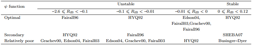
As described above,a large number of hydrometeorological observations from the tower platform near Xisha Isl and are employed to investigate the validity of different ψ functions based on three comparison criteria,together with the latest forms of ψ functions.The results show that the validity of ψ functions is closely related to the stratification indicated by the values of RiB,as shown in Table 1.For unstable conditions of-2.6 6 RiB <-0.1,the optimal function is Fairall96;for weak unstable conditions of-0.1 6 RiB < -0.01,Fairall96 is second only to HYQ92; and for nearneutral but slightly unstable conditions of-0.01 6 RiB < 0,the effects of Edson04,Fairall03,Grachev00, and Fairall96 are very similar,with the best(Edson04)offering only a very weak advantage.Therefore,the Fairall96 function offers optimal performance overall,although it is difficult to determine a fixed ψ function that performs best across the entire stability range of -2.6 6 RiB < 0.Under stable conditions,HYQ92 performs best with an obvious advantage,followed by the newly introduced SHEBA07 nonlinear function.As a result,the optimal Fairall96(for unstable conditions) and HYQ92(for stable conditions)are here incorporated into the UED model to obtain a newly improved model,namely the UED_F96_H92 model.
 |
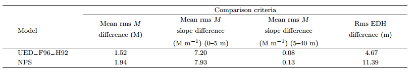
Comparison of the model performance in calculating M,M slope, and EDH between the UED F96 H92 model and the NPS model is undertaken based on 2143 sets of measured data and the three objective criteria mentioned above.The results are shown in Fig. 12 and Table 2.For conditions of RiB < 0,the UED F96 H92 model performs slightly better than NPS model in calculating M values;conversely,for RiB > 0,this model can reduce the rms M differences from above 8 M to about 2 M.For the M slope of 0-5 m,the UED _F96_H92 model performs better than NPS model throughout the entire stratification range except 0 6 RiB < 0.06.Moreover,it is superior to the NPS model in calculating M slope for 5-40 m,especially under stable conditions.For conditions of-2.6 6 RiB <-0.2,the model-derived EDHs from the above two models are both lower than the curve-fit values,with the values from the UED _F96_H92 model being much closer to the observations.When RiB varies from-0.2 to 0,the EDHs from the UED F96 H92 model fluctuate around the curve-fit values,whereas those from the NPS model are consistently lower than the observations.When stratification becomes stable,the EDHs from the NPS model increase sharply with RiB;these unreasonably high EDHs can be inhibited successfully by the improved UED F96 H92 model,but the resultant EDHs are still higher than the observations.Considering the mean effects of all 2143 sets of data,the UED F96 H92 model is found to have reduced the calculated mean rms M difference,mean rms M slope difference for 0-5 and 5-40 m, and rms EDH difference by 21.65%,9.12%,38.79%, and 59.06%,respectively,when compared to the NPS model.
 |
| Fig. 12. Scatter plots of the (a) rms M difference,(b)0-5-m rms M slope difference,(c)5-40-m rms M slope difference, and (d) EDH difference (model minus observation) between the UED_F96_H92 model and the NPS model versus RiB. |
This paper aimed to validate the performance of the various forms of stability(ψ)functions in the unified evaporation duct(UED)model that was proposed in Part I of this study.The ψ function is the key factor affecting the UED model performance.In particular,the study aimed to determine the most favorable ψ functions applicable to specific sea area and stratification conditions and then introduce them into the UED model,thus allowing improvements to duct models.To achieve this objective,a large number of hydrometeorological observations from a tower platform over Xisha Isl and of the South China Sea were employed,together with the latest proposed forms of ψ functions.The validity of different ψ functions for specific stratifications was investigated based on three comparison criteria.
The results show that,for conditions of-2.6 6 RiB <-0.1,Fairall96 performs best in calculating M,M slope, and EDH,followed by HYQ92.The performances of other functions including Grachev00,Edson04, and Fairall03 are relatively poor owing to their underestimation of EDHs.This implies that the improvements to the COARE algorithm itself pose some limitations;although the newer COARE 2.6 and COARE 3.0 use Grachev00 and Fairall03 instead of Fairall96,their performance in estimating evaporation ducts over the selected observation station in the tropical Pacific Ocean is poorer than that of Fairall96. Moreover,as conditions become weakly unstable(-0.1 6 RiB <-0.01),Fairall96 performs second best to HYQ92;conversely,for near-neutral but slightly unstable conditions(-0.01 6 RiB < 0.0),the effects of Edson04,Fairall03,Grachev00, and Fairall96 are very similar,with the best function(Edson04)offering only a very weak advantage.On this occasion,the performance of HYQ92 is considered to be relatively poor owing to its overestimation of the EDHs.Under stable conditions,HYQ92 is the optimal function with an obvious advantage,followed by the newly introduced SHEBA07.
Based on these results,the most favorable functions,i.e.,Fairall96 and HYQ92,have been incorporated into the UED model to obtain an improved model.This model was able to reduce the calculated mean rms modified refractivity(M)difference,mean rms M slope difference for 0-5 and 5-40 m, and rms EDH difference by 21.65%,9.12%,38.79%, and 59.06%,respectively,when compared to the NPS model.Nevertheless,our results must be confirmed further by more observation cases,particularly because our study relies on a single source of measured data,obtained primarily from the sea area near the Xisha Isl and .
Acknowledgments.We are very grateful to the reviewers of this article for their insightful comments and suggestions.
| Babin, S. M., G. S. Young, J. A. Carton, et al., 1997: A new model of the oceanic evaporation duct. J. Appl. Meteor., 36, 193-204. |
| Babin, S. M., and G. D. Dockery, 2002: LKB-based evaporation duct model comparison with buoy data. J. Appl. Meteor., 41, 434-446. |
| Cheng, Y. G., and W. Brutsaert, 2005: Flux-profile relationships for wind speed and temperature in the stable atmospheric boundary layer. Bound.-Layer Meteor., 114, 519-538. |
| Cook, J., 1991: A sensitivity study of weather data inaccuracies on evaporation duct height algorithms. Radio Sci., 26, 731-746. |
| Dai Fushan, Li Qun, Dong Shuanglin, et al., 2002: Atmospheric Duct and Its Military Application. PLA Press of China, Beijing, 153-243. (in Chinese) |
| Ding Juli, Fei Jianfang, Huang Xiaogang, et al., 2009: Contrast study on the occurrence of evaporation ducts in the South China Sea and East China Sea. Chinese J. Radio Sci., 24, 1018-1023. (in Chinese) |
| Ding Juli, Fei Jianfang, Huang Xiaogang, et al., 2011: Improvement to the evaporation duct model by introducing nonlinear similarity functions in stable conditions. J. Trop. Meteor., 27, 410-416. |
| Ding Juli, Fei Jianfang, Huang Xiaogang, et al., 2015: Development and validation of an evaporation duct model. Part I: Model establishment and sensitivity experiments. J. Meteor. Res., 29, 467-481, doi: 10.1007/ s13351-015-3238-3. |
| Fairall, C. W., E. F. Bradley, D. P. Rogers, et al., 1996: Bulk parameterization of air-sea fluxes for Tropical Ocean-Global Atmosphere Coupled-Ocean Atmosphere Response Experiment. J. Geophys. Res., 101, 3747-3764. |
| Frederickson, P. A., K. L. Davidson, C. R. Zeisse, et al., 2000: Estimating the refractive index structure parameter over the ocean using bulk methods. J. Appl. Meteor., 39, 1770-1783. |
| Gehman, J. Z., 2000: Importance of Evaporation Duct Stability in Propagation-Sensitive Studies. JHU/APL Technical Report, A2A-00-U-3-008, 8 pp. |
| Grachev, A. A., E. L. Andreas, and C. W. Fairall, 2007: SHEBA flux-profile relationships in the stable atmospheric boundary layer. Bound.-Layer Meteor., 124, 315-333. |
| Hu Yinqiao and Zhang Qiang, 1992: Local similarity in the atmosphere boundary layer. Chinese J. Atmos. Sci., 17, 10-20. (in Chinese) |
| Ivanov, V. K., V. N. Shalyapin, and Y. V. Levadnyi, 2007: Determination of the evaporation duct height from standard meteorological data. Atmos. Ocean. Phys., 43, 36-44. |
| Jeske, H., 1973: State and limits of prediction methods of radar wave propagation conditions over the sea. Modern Topics in Microwave Propagation and Air-Sea Interaction, A. Zancla, Ed., D. Reidel Publishing, 130-148. |
| Katzin, M., R. W. Bauchman, and W. Binnian, 1947: 3and 9-centimeter propagation in low ocean ducts. Proceedings of the IRE, 35, 891-905. |
| Li Yunbo, Zhang Yonggang, Tang Haichuan, et al., 2009: Oceanic evaporation duct diagnosis model based on air-sea flux algorithm. J. Appl. Meteor. Sci., 20, 628-633. (in Chinese) |
| Liu Chengguo, Huang Jiying, Jiang Changyin, et al., 2001: Modeling evaporation duct over sea with pseudo-refractivity and similarity theory. Acta Electron. Sinica, 29, 970-972. (in Chinese) |
| Liu Chengguo, 2003: Research on evaporation duct propagation and its applications. Ph. D. dissertation, University of Xidian, China, 124 pp. (in Chinese) |
| Liu, W. T., and T. V. Blanc, 1984: The Liu, Katsaros and Businger (1979) Bulk Atmospheric Flux Computational Iteration Program in FORTRAN and BASIC. NRL Memorandum Report 5291, 8 May 1984, AD-A156, 736. |
| Musson-Genon, L., S. Gauthier, and E. Bruth, 1992: A simple method to determine evaporation duct height in the sea surface boundary layer. Radio Sci., 27, 635-644. |
| Pan Yue and Cui Wei, 2007: Study on the application of PJ evaporation duct model in coastal region. Computer Simulation, 24, 86-89. |
| Pasricha, P. K., M. V. S. N. Prasad, and S. K. Sarkar, 2002: Comparison of evaporation duct models to compute duct height over Arabian sea and Bay of Bengal. Indian J. Radio & Space Physics, 31, 155158. |
| Paulus, R. A., 1985: Practical application of an evaporation duct model. Radio Sci., 20, 887-896. |
| Stull, R. B., 1991: An Introduction to Boundary Layer Meteorology. Klawer Academic Publishers, America, 40-45. |
| Tian Bin, Cha Hao, Zhang Yusheng, et al., 2009: Study on the applicability of evaporation duct model A in Chinese sea areas. Chinese J. Radio Sci., 24, 556-561. |
| Webb, E. K., 1970: Profile relationships: The log-linear range and extension to strong stability. Quart. J. Roy. Meteorol. Soc., 96, 67-90. |
| Yaglom, A. M., 1977: Comments on wind and temperature flux-profile relationships. Bound.-Layer Meteor., 11, 89-102. |
| Yagüe, C., S. Viana, G. Maqueda, et al., 2006: Influence of stability on the flux-profile relationships for wind speed, φm, and temperature, φh, for the stable atmospheric boundary layer, Nonlin. Processes Geophys., 13, 185-203. |
| Yang Kunde, Ma Yuanliang, and Shi Yang, 2009: Spatiotemporal distributions of evaporation duct for the West Pacific Ocean. Acta Phys. Sinica, 58, 73397350. (in Chinese) |
| Zhang Qiang and Hu Yinqiao, 1995: The flux-profile relationships under the condition of heat advection over moist surface. Scientia Atmospherics Sinica, 19, 8-19. (in Chinese) |
| Zuo Lei, Cha Hao, Tian Bin, et al., 2009: An initial study on the applicability of Paulus-Jeske model of evaporation duct in Chinese sea areas. Acta Electron. Sinica, 37, 1100-1103. (in Chinese) |