 2015, Vol. 29
The Chinese Meteorological Society
Article Information
- LI Chao, CHEN Dehui, LI Xingliang, HU Jianglin. 2015.
- Effects of Terrain-Following Vertical Coordinates on High-Resolution NWP Simulations
- J. Meteor. Res., 29(3): 432-445
- http://dx.doi.org/10.1007/s13351-015-4212-x
Article History
- Received September 17, 2014;
- in final form December 30, 2014


2 University of Chinese Academy of Sciences, Beijing 100049;
3 Numerical Weather Prediction Center, China Meteorological Administration, Beijing 100081
Topography plays a significant role in the general circulation of the atmosphere due to its dynamical and thermodynamical forcing effects.Chen et al.(2008)pointed out that lee vortices and shear lines generated by mountain waves are important weather systems,which can induce mesoscale rainfall events.Effects of surface boundary friction also contribute to the rainfall process.The mountain waves are often accompanied by blocking flows and flows around and across the mountains.Low-level jets generated by the combination of dynamic and thermodynamic topographic effects provide an efficient way for water vapor transport and thus play a critical role for the triggering and sustaining of the precipitation process.The topographic effects also affect frontogenesis,frontolysis,occluded fronts, and the circulation pattern of fronts. Changes in the path and intensity of tropical cyclones caused by topographic forcing will eventually affect the intensity and predicted area of precipitation.Various scales of topographies have different effects on the weather and climate of China.For example,the dynamic and thermodynamic forcing of the Tibetan Plateau(TP)can significantly modify the synoptic weather systems that move into this area, and induce various synoptic phenomena downstream of the TP(Ye et al., 1979).The thermodynamic effects of the TP have an important impact on the movement and development of the East Asian trough,which provides the large-scale background for a variety of mesoscale systems.The southwest vortex and low-level jet occurring downstream of the TP are two important systems that control the precipitation in Southwest China.In addition,the dynamic effects of small-scale mountains such as the Qin Mountains have pronounced impacts on local convection(Li et al., 2012a).In order to improve the accuracy in weather forecasting,numerical weather prediction models must correctly describe the influence of the topographic forcing.The vertical coordinate of the numerical model is directly related to physical and dynamical processes over complex terrain area.The equations can be simplified dramatically if written in an appropriate coordinate system,allowing the application of simpler and more accurate solving techniques and better description of lower boundary conditions.Computational errors such as the pressure gradient force(PGF)error and other errors associated with the horizontal difference can be reduced and the model performance can be improved if an appropriate formulation of vertical coordinate is chosen.
Increasing resolution is one of the most efficient methods to improve the capability of numerical weather prediction models.With the increase in the resolution of numerical weather prediction models,the topography can be described with finer resolution and thus the steep terrain slopes will become more realistic in the model.However,the traditional terrain-following vertical coordinate proposed by GalChen and Somerville(1975;hereinafter referred to as the Gal.C.S coordinate)would cause an increase in the PGF error and result in serious distortion of the gravity waves over terrains of steep slope.In this sense,the negative effects of the Gal.C.S coordinate in the high-resolution numerical simulations are quite distinct,making it inappropriate for high resolution modeling studies.The coordinate currently used in the GRAPES-Meso model,which is independently developed by China Meteorological Administration,still uses the Gal.C.S coordinate mentioned above,but with a substantial modification.The original sigma-z vertical formation for the Gal.C.S coordinate is expressed as:
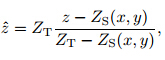
 are the absolute and relative heights of the coordinate surface,ZS is the topographic height, and ZT is the top of the upper boundary layer.This type of coordinate allows the model to calculate in a "rectangular" bounded domain and facilitates the programming.Moreover,the irregular lower boundary in the real atmosphere is transformed into a smooth,terrain-following lower boundary,which greatly simplifies the calculation of the lower boundary condition for the model.Since this approach allows for unequal spacing in the computational levels,it provides a simple method to couple the dynamical part of the atmospheric prediction model with the planetary boundary layer and surface layer parameterization schemes(Phillps,1957).As a result,the dynamic and thermodynamic effects of the terrain forcing can propagate properly to the upper atmosphere.However,there exist serious deficiencies in the Gal.C.S coordinate system despite its beneficial effects in the calculation of surface and boundary layer processes. Strictly speaking,the Gal.C.S coordinate system is not an orthogonal coordinate system(Zdunkowski and Bott, 2003);consequently,the original PGF that is derived from one term has to be calculated based on small differences between two terms due to the coordinate transformation.This inevitably results in the PGF errors.The airflow along the coordinate surfaces deviates from quasi-horizontal flow in the upper atmosphere even though the terrain effect decays gradually from the bottom to the top.With an increasing model resolution,the terrain slope that the Gal.C.S coordinate needs to follow becomes steeper.This causes significant distortions in the simulated gravity wave. Li et al.(2012b)pointed out that errors in both the PGF and the mass advection dissipation using the onescale smoothed level(SLEVE1),two-scale smoothed level(SLEVE2)(Schär et al., 2002), and the COSINE(COS)coordinates are all significantly reduced in comparison with those using the Gal.C.S coordinate.To successfully develop the GRAPES-Meso model,the design of the vertical coordinate is a critical issue. A series of ideal testing cases such as testing of the gravity wave simulation under complex terrain area,testing of pressure gradient force calculation with real topography, and operational bulge testing have been conducted using the GRAPES-Meso model to compare the four coordinates proposed by Li et al.(2012b). The purpose of this study is to analyze the operational test results and determine a vertical coordinate scheme,which can reduce the PGF errors and improve the forecasting accuracy of the high-resolution mesoscale model.
2. Coordinates in common formulation
are the absolute and relative heights of the coordinate surface,ZS is the topographic height, and ZT is the top of the upper boundary layer.This type of coordinate allows the model to calculate in a "rectangular" bounded domain and facilitates the programming.Moreover,the irregular lower boundary in the real atmosphere is transformed into a smooth,terrain-following lower boundary,which greatly simplifies the calculation of the lower boundary condition for the model.Since this approach allows for unequal spacing in the computational levels,it provides a simple method to couple the dynamical part of the atmospheric prediction model with the planetary boundary layer and surface layer parameterization schemes(Phillps,1957).As a result,the dynamic and thermodynamic effects of the terrain forcing can propagate properly to the upper atmosphere.However,there exist serious deficiencies in the Gal.C.S coordinate system despite its beneficial effects in the calculation of surface and boundary layer processes. Strictly speaking,the Gal.C.S coordinate system is not an orthogonal coordinate system(Zdunkowski and Bott, 2003);consequently,the original PGF that is derived from one term has to be calculated based on small differences between two terms due to the coordinate transformation.This inevitably results in the PGF errors.The airflow along the coordinate surfaces deviates from quasi-horizontal flow in the upper atmosphere even though the terrain effect decays gradually from the bottom to the top.With an increasing model resolution,the terrain slope that the Gal.C.S coordinate needs to follow becomes steeper.This causes significant distortions in the simulated gravity wave. Li et al.(2012b)pointed out that errors in both the PGF and the mass advection dissipation using the onescale smoothed level(SLEVE1),two-scale smoothed level(SLEVE2)(Schär et al., 2002), and the COSINE(COS)coordinates are all significantly reduced in comparison with those using the Gal.C.S coordinate.To successfully develop the GRAPES-Meso model,the design of the vertical coordinate is a critical issue. A series of ideal testing cases such as testing of the gravity wave simulation under complex terrain area,testing of pressure gradient force calculation with real topography, and operational bulge testing have been conducted using the GRAPES-Meso model to compare the four coordinates proposed by Li et al.(2012b). The purpose of this study is to analyze the operational test results and determine a vertical coordinate scheme,which can reduce the PGF errors and improve the forecasting accuracy of the high-resolution mesoscale model.
2. Coordinates in common formulation
As discussed in Li et al.(2012a),the new general coordinate form is given as:
where i denotes different scales of terrain. When L = 1,the vertical decay function is expressed as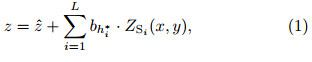
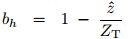 for the Gal.C.S coordinate, and
 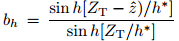 for the SLEVE1 coordinate. The decay function for the COS coordinate is
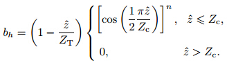
When L = 2,the vertical decay functions for
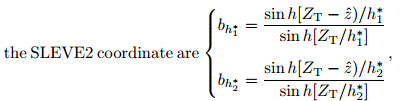
The general coordinate form Eq.(1)divides the absolute height of the coordinate surface into the relative height and the effect of the terrain.Each different coordinate has its corresponding terrain attenuation coefficient that controls the decaying rate.The SLEVE2 coordinate should be regarded as an improvement on the SLEVE1.The SLEVE2 uses the scaledependent coefficient that decays with height of the underlying terrain to generate a much smoother computational mesh.The COS,obtained from the coordinate form proposed by Klemp(2011),is tested herein to further smooth the upper coordinate surfaces until the topographic features vanish on the upper levels.The following formula deductions and tests are all based on the coordinate forms described above.
3. The GRAPES-Meso dynamical core with the general coordinateThe terrain-following coordinate is closely related to calculation of the PGF,vertical velocity,divergence, and other physical quantities in the model dynamical core.We will deduce the equations and the physical quantities of the model framework using the general coordinate without special consideration.
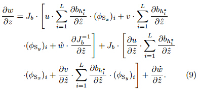
For the vertical velocity,the numerical partial derivatives with respect to time are transformed on both sides of Eq.(1):
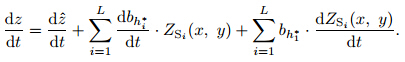
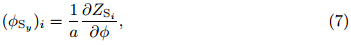
 is the vertical velocity expressed in the form of reference of the general coordinate. φSx and φSy are the slopes of the terrain along x and y directions, and
 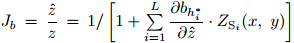 is the Jacobian of the transformation.
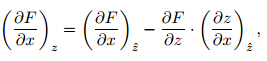
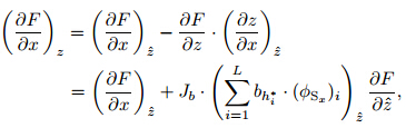
The coordinate transformation involves vertical and horizontal partial derivatives. The horizontal derivative with respect to x(with “x” being an example)is transformed according to the equation below:
The horizontal relations are then written as:
Thus,the PGF is calculated as
where φSi = gZSi is the terrain potential height.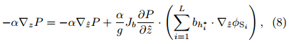
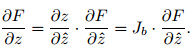
From the horizontal partial derivatives,we can obtain:
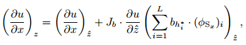
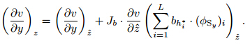
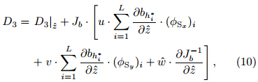
The above derivatives clearly indicate that,in order to correctly apply the general coordinate in the model dynamic core,these terms must be transformed appropriately with regard to the terrain in model domain. Different values of Jb and b are required for the corresponding coordinates. There are other formulas related to the terms mentioned above that also need to be reconstructed,such as linear and nonlinear terms, and the coefficient of the Helmholtz equation(Xue et al., 2008).
4. Idealized cases of gravity wave simulationMountains with different scales generate gravity waves of various patterns,which induce a wide variety of weather conditions because of their complex structure.Herein,we conduct the mountain wave experiments to evaluate the simulation of gravity waves using the four coordinates.The basic state of the atmosphere is featured by a constant mean flow of U= 10 m s−1, and a uniform stratification with a BruntVaisala frequency N=0.01.The reference potential temperature at the surface is 280 K.
The ideal terrain is a mixture of the bell-shape and small-scale terrain,which is defined as ZS= 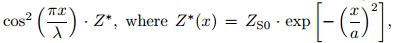 ZS0=250 m,λ=4 km, and a=5 km.In this case,λ is the wavelength of the small-scale terrain;a is the horizontal span of the terrain, and is also half the length of the large-scale terrain that has a wavelength of 2πa.Gravity waves with two different scales will be generated by the mountain forcing:large-scale hydrostatic waves that propagate vertically over the entire domain, and small-scale waves that decay rapidly with height due to the non-hydrostatic effect(Anther and Warner, 1978).Assuming a/λ to be fixed,the gravity waves simulated in the frictionless and adiabatic atmosphere are controlled by two dimensionless quantities:Nh0/U and Na/U.Thus,the final result is only connected with the terrain scale if N/U is given.
The computational domain covers an area of(-25000,25000)m ×(0,21000)m with a grid spacing of δx=250 m in x direction and δζ=210 m in ζ direction.No-flux boundary conditions are used for the bottom boundary, and non-reflecting boundary conditions are imposed by a sponge layer of 9 km for the top boundary and a relaxation zone of 1 km for the lateral outflow boundary.
The mountain for the SLEVE2 coordinate is divided into large-scale component Zh1∗ and small-scale component Zh2∗,which are defined as follows:
where h∗= 8 km,h1∗ = 8 km,h2∗ = 1.5 km,Zc = 8 km, and n = 4. In the ideal test cases,we define the terrain according to the above formulas since the terrain in the ideal cases is quite regular and can be well described by these formulas. Note that in the real data testing cases,the topographic splitting should be obtained using the Laplace smoothing digital filter. We will introduce details of the splitting method in the simulation with realistic terrain in the next section.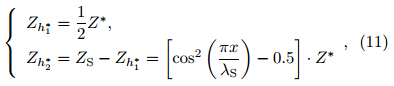
Vertical cross-sections of four coordinate planes are shown in Fig. 1.Note that the topographic effects of the three smoothed level coordinates at different levels are smaller than that of Gal.C.S coordinate.The small-scale perturbations on the SLEVE2 surfaces are gradually smoothed from the bottom to 3 km compared with that in the SLEVE1 coordinate, and the large-scale perturbations decay slowly.In addition,the COS surfaces become completely flat above 8 km. Although the large-scale fluctuations in the SLEVE2 surfaces are still evident above 8 km,the influence of the small-scale terrain at lower levels is smaller than that at the corresponding levels in the COS coordinate.Testing results of gravity wave simulation along these different coordinate planes will be discussed in the next.
 |
| Fig. 1. Vertical cross-sections showing four distributions of vertical coordinate planes. (a) The Gal.C.S coordinate, (b) the SLEVE1 coordinate, (c) the SLEVE2 coordinate, and (d) the COS coordinate. |
Figure 2 shows the comparison of the vertical velocity using the four coordinates and the analytic solution for a steady-state flow over the same mountain after 10 h.The semi-analytic solution based on the linear theory is obtained with a Fourier transformation(Smith, 1979,1980).The results indicate that the patterns of the gravity waves can basically be simulated correctly in all the four coordinates,except that the non-hydrostatic components generated by the smallscale terrain show some differences.However,the influence of terrain on the coordinate planes results in dramatically distorted unphysical wave patterns at upper levels;the error in the Gal.C.S coordinate(Fig. 2b)is especially pronounced compared to the linear analytic solution(Fig. 2a).The distortion of the wave pattern is caused by the mixing of hydrostatic waves and decaying non-hydrostatic waves.It is worth noting that the small-scale non-hydrostatic waves are damped with height at various extents in the three smoothed level coordinates.The results simulated in the SLEVE2 coordinate(Fig. 2d)show excellent agreement with the analytic solution.At lower levels,the small-scale terrain effect decays with height more slowly in the COS coordinate(Fig. 2e)than in the SLEVE2 coordinate.As a result,small-scale wave patterns are more obvious in the COS coordinate than in the SLEVE2 coordinate.However,the vertical velocity in the COS coordinate is smaller than that in the SLEVE2 coordinate between 6- and 10-km heights,where the COS coordinate planes become flat.
 |
| Fig. 2. Comparison of the vertical velocity of the four coordinates and the analytic solution for the steady-state flow over mountain after 10 h. The time step is 0.3 s and the contour interval is 0.05 m s−1. (a) The analytic solution, (b) the Gal.C.S, (c) the SLEVE1, (d) the SLEVE2, and (e) the COS coordinates. |
Given all the test results,it is clear that the model using smoothed level coordinates can provide higher accuracy in the gravity wave simulations than that using the Gal.C.S coordinate.Considering the fact that the simulation with the SLEVE2 coordinate agrees best with analytical solution.The SLEVE2 coordinate is taken as the most appropriate coordinate for the GRAPES-Meso model.
5. Application and simulation using the GRAPES-Meso modelThe smoothed level coordinates are proved to be appropriate based on results of both theoretical analyses and ideal testing cases.To further investigate the model performance using this type of vertical coordinate,we adopt the smoothed level coordinates in the GRAPES-Meso model and conduct a suite of simulations using real topography within the model domain. First,we compare the idealized PGF calculation errors using the four coordinates and real topography.Second,bulge simulations are carried out with real data to assess the comprehensive forecasting capability of the model using the four coordinates.The model used here is the GRAPES-Meso version 3.2 with a horizontal resolution of 0.15° × 0.15°.The number of vertical levels is 33 and the time step is 90 s.The initial and boundary fields are extracted from the NCEP 1° × 1° reanalysis data.The model domain covers 15°-64.35°N,70°-145.15°E, and the simulations are performed without data assimilation.
5.1 PGF error in ideal test cases with real topographyWe compare the PGF errors at various levels in a suite of ideal test cases using different coordinates.The vertical layers are calculated based on real topography.The coordinate transformation of SLEVE1/2 and COS is under control of parameters such as h1∗,h2∗,n, and Zc(Li et al., 2012b).Considering the maximum height of the topography,we set h∗= 10 km,h1∗=10 km,h2∗=3 km,Zc=11.6 km, and n=3 to satisfy the coordinate invertibility conditions and ensure computational stability.
The filter scheme for SLEVE2 is given by
where m is the number of filters used(set at 100),subscripts i and j denote the longitude and latitude grid indices,respectively, and β is the coefficient of the filter. Here we set β = 0.2.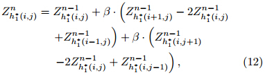

Figure 3 shows cross-sections of the coordinate planes along 34°N for the four coordinates using the parameters set previously.Note that the specific terrain features and mountain peaks are clearly visible in the coordinate surface of the Gal.C.S coordinate. However,the characteristic amplitude of the terrain is less distinct(to various degrees)at the middle and upper levels in the SLEVE1,SLEVE2, and COS coordinates in comparison with that in the Gal.C.S coordinate.Compared to that in the SLEVE1 coordinate,the small-scale terrain variation in the SLEVE2 coordinate is filtered layer by layer,suggesting that the small-scale noise along the coordinate surfaces is rapidly damped with height in the SLEVE2 coordinate.For the COS coordinate,the coordinate surfaces have not become flat until 11.6 km, and the layer thickness is significantly reduced below this height.
 |
| Fig. 3. Vertical cross-sections showing the vertical coordinate distributions along 34°N in the GRAPES-Meso model. (a) The Gal.C.S coordinate, (b) the SLEVE1 coordinate, (c) the SLEVE2 coordinate, and (d) the COS coordinate. |
Theoretically,the analytic value of the PGF error is zero when calculated under the reference atmosphere state because of the uniform pressure field. Therefore,the discretized PGF value is the PGF error.The reference atmosphere is given by Eq.(12), and the PGF is calculated from Eq.(13)using the classical algorithm(Qian and Zhou, 1995).
Figure 4 shows the PGF errors along the meridional direction at lower(about 1 km),middle(about 6 km), and upper(about 15 km)levels respectively for the four coordinates.The PGF errors all occur upon the area of steep topography, and decay with height. The errors in the SLEVE1 and SLEVE2 coordinates are smaller than that in the Gal.C.S coordinate at the same level,which agree well with the distribution of the coordinate planes.Moreover,the PGF error in the COS coordinate is not present at upper levels,whereas it is more obvious than that in the Gal.C.S coordinate at the lower levels.Because the small-scale noises in the SLEVE2 coordinate are significantly damped at middle and upper levels,the PGF error is smaller in the SLEVE2 coordinate than that in the SLEVE1 coordinate at the same level.These findings are in good agreement with results of the previous tests using the ideal vertical layer and topography(Li et al., 2012b). In general,the PGF errors in several smoothed level coordinates are reduced to various extents.Furthermore,despite the increase in the PGF errors at lower levels in the COS coordinate,the improved performance at high levels cannot be ignored.
 |
| Fig. 4. Comparison of the PGF error from the ideal test with Gal.C.S, SLEVE1, SLEVE2, and COS coordinates at (a1, b1, c1, and d1) lower levels; (a2, b2, c2, and d2) middle levels, and (a3, b3, c3 and d3) upper levels. The shaded area indicates the topography. |
To evaluate the operational forecast capability of the model by using the four coordinate systems,an operational bulge test is carried out.The test lasts for 30 days,from 0800 LT(local time)1 to 0800 LT 30 September 2013,with a 48-h rolling forecast every day. The parameters are set to be the same as those in the ideal test cases described in the previous section.The operational forecast of the geopotential height,temperature, and wind are described below.
The errors generated by the TP follow the airflow to propagate to downwind areas.Thus,the propagation tracks and locations of the accumulated errors differ with various stream patterns at different vertical levels.The average bias of the geopotential height at 100 hPa is shown in Fig. 5.The westerly wind belt at this level is almost straight with slight troughs and ridges.The biases in the four coordinates are quite distinct and different from each other above the Hetao area.The maximum bias in the SLEVE2 coordinate is the smallest,less than that in the Gal.C.S coordinate by more than 16 gpm.The second smallest bias of geopotential height is found in the SLEVE1 coordinate.The bias in the COS coordinate is between those in the SLEVE2 and Gal.C.S coordinates.Theoretically,the coordinate surfaces in the COS coordinate should have flattened at 16-km height,i.e.,the geometrical height of 100 hPa;however,the actual simulation results do not reflect the advantages of the flattened model surfaces in the COS coordinate compared to that in the SLEVE2 coordinate.The largest bias at 500 hPa(Fig. 6)is found to the east of the TP,where three provinces(Sichuan,Qinghai, and Gansu)converge.The TP has an altitude of approximately 500 hPa,where the westerly trough is deeper than that at 100 hPa.As a result,the errors are brought to inl and China following the airflow, and the errors are especially distinct in the area downwind of the TP. The biases in the SLEVE1 and SLEVE2 coordinates are still smaller than that in the Gal.C.S coordinate,but errors in the COS coordinate are a little larger than that in the Gal.C.S coordinate.The bias at 850 hPa(Fig. 7)is partly masked by the TP.The main error lies in the Sichuan basin,where southwest vortexes form.The model using the SLEVE2 coordinate performs best,while the model performance with the COS coordinate is similar to that with Gal.C.S coordinate.
 |
| Fig. 5. Average deviation of the 48-h height (gpm) forecast in the bulge test against FNL reanalysis data at 100 hPa. (a) The Gal.C.S coordinate, (b) the SLEVE1 coordinate, (c) the SLEVE2 coordinate, and (d) the COS coordinate. |
 |
| Fig. 6. As in Fig. 5, but at 500 hPa. |
 |
| Fig. 7. As in Fig. 5, but at 850 hPa. |
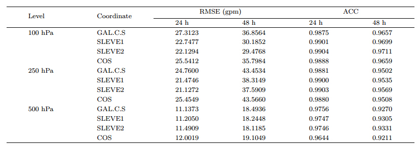
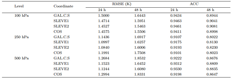
The statistical analysis of different variables directly demonstrates the forecasting capability.For further comparison,Tables 1 and 2 give the statistical results of root mean square error(RMSE) and anomaly correlation coefficient(ACC)of the geopotential height and temperature in the bulge test.The RMSEs of the geopotential height at 100 and 250 hPa for the SLEVE1 and SLEVE2 coordinates are remarkably small at 48-h forecast compared to that for the Gal.C.S coordinate.The RMSE is particularly small in the SLEVE2 coordinate.The RMSE at 100 hPa is slightly smaller in the COS coordinate than that in the Gal.C.S coordinate.However,the results are quite similar at the lower levels.Moreover,results with the SLEVE1 and SLEVE2 coordinates are more consistent with observations than that with the Gal.C.S coordinate.Again,with a large ACC at 500,250, and 100 hPa,the model using the SLEVE2 coordinate gives the best result.Statistical analysis of temperature gives generally similar conclusion to that for the geopotential height,as shown in Table 2.The SLEVE2 coordinate performs the best.The COS coordinate has some deficiencies compared with the Gal.C.S coordinate at some levels,but is close to the SLEVE2 coordinate at 100 hPa.
 |
The biases of the average meridional wind at 850 hPa are shown for the four coordinates in Fig. 8.The main area of large bias is located downstream of the TP,such as in eastern Sichuan Province and most of Chongqing.The biases are reduced more or less in southeastern China in all the coordinates except for the COS coordinate.The meridional wind is closely linked to atmospheric water vapor transport,thus improvement in the meridional wind prediction will definitely be favorable for accurate precipitation forecast. The operational forecast results of the GRAPES-Meso model show that the simulated meridional wind in East Asia is often larger than the observed values.The results of the present study clearly indicate that the smooth-level coordinates,particularly SLEVE2,can help to solve the problem.
 |
| Fig. 8. As in Fig.7, but for meridional wind (m s−1) forecast. |
In summary,the SLEVE2 coordinate is better than the other three coordinates discussed in this study.Errors in both temperature and geopotential height simulations are reduced by using the SLEVE2 coordinate, and the operational forecast capacity of the model using this coordinate gives the best result compared to that using the other three coordinates.
Figure 3d shows that the thickness of the bottom layers over the TP are compressed sharply in the COS coordinate.Theoretically,there should have better simulations at levels above 100 hPa,which are high above the critical attenuation height of the COS coordinate.However,the actual results are contradictory to this theoretic assumption.The reason for this result is probably because the critical attenuation height is too low.As a result,the thickness of the lower model layers over the TP is far too thinner than that over the plain areas to the east of the Tibet at the same latitude,which eventually induces large differences in the accuracy of model integration in different areas. We have not obtained promising results for the COS coordinate in this study.Further research will be conducted to address this issue in our future studies.
6. ConclusionsTo investigate the impact of the design of vertical coordinate on model performance,we have conducted a series of tests and analysis,i.e.,ideal testing cases for gravity wave simulation,PGF error analysis under real topography, and the operational bulge test using the GRAPES-Meso model with four different coordinate systems.The preliminary conclusions are as follows.
(1)The results of the ideal test cases for gravity wave simulation show that the pattern and vertical structure of the gravity wave can be well simulated by the model using the four coordinates.However,the distortion of the wave can be effectively eliminated in the three smoothed-level coordinates but not in the Gal.C.S coordinate.Moreover,for the SLEVE2 and COS coordinates,the outputs are very close to the analytic solutions at middle and upper levels.However,for the COS coordinate,noticeable topographic features at the base are still distinct.
(2)The PGF errors with real topography in the SLEVE1 and SLEVE2 coordinates are smaller than that in the Gal.C.S coordinate at each level, and the model performance with SLEVE2 coordinate is better than that with the SLEVE1.The errors in the COS coordinate disappear at higher levels,but are obvious at lower levels compared to that in the Gal.C.S coordinate.The coordinate surfaces of SLEVE2 at upper levels are nearly as smooth as those of the COS coordinate, and the errors at the upper levels can almost be ignored.
(3)The one-month real-data simulation using the GRAPES-Meso model with the SLEVE1 and SLEVE2 coordinates gives similar results regarding to the PGF error tests.The largest improvement is observed at 850,500, and 100 hPa,with a decrease in both the bias and RMSE of the geopotential height and the temperature, and an increase in the ACC.Among the four coordinates discussed in this study,the SLEVE2 coordinate gives the best results.However,the model results for real-data case using the COS coordinate are not as promising as in the ideal test,with advantages only occurring at the highest 100 hPa.Analysis of the bias of the meridional wind simulation also suggests that the three smooth-level coordinates are superior to the COS coordinate, and the SLEVE2 coordinate is particularly appropriate for the GRAPES-Meso model.Altogether,the simulation capability of the GRAPES-Meso model with the SLEVE2 coordinate is the most promising for operational forecast.
To solve the problem caused by the excessively thin layers in the COS coordinate,Klemp(2011)proposed a smoothing method based on this coordinate. This method both smoothes the terrain using the attenuation coefficient b and filters the terrain layer by layer.It actually consists of the merits of the SLEVE2 and the COS coordinates.In future studies,we will investigate the impact of the new coordinate and seek to solve the problems existing in the current COS coordinate.Note that the analysis of the testing results in the present study is not complete.We will further analyze the impact of the smoothed-level coordinate on airflow and water vapor transport in our future study.
Acknowledgments.Zhou Feifei is gratefully acknowledged for her help with statistical calculation of the bulge test result.
| Anther, R. A., and T. T, Warner, 1978: Development of hydrodynamic models suitable for air pollution and other meso-meteorological studies. Mon. Wea. Rev., 106, 1045-1078. |
| Chen Dehui, Xue Jishan, Yang Xuesheng, et al., 2008: New generation of multi-scale NWP system (GRAPES): General scientific design. Chin. Sci. Bull., 53, 3433-3445. |
| Gal-Chen. T. J., and R. C. Somerville, 1975: On the use of a coordinate transformation for the resolution of the Navier-Stokes equation. J. Comput. Phys., 17, 209-228. |
| Klemp, J. B., 2011: A terrain-following coordinate with smoothed coordinate surfaces. Mon. Wea. Rev., 139, 2163-2169. |
| Li Chao, Li Xingliang, and Chen Dehui, 2012a: Impact of height-based terrain-following coordinates on a case of heavy rain simulations. Torrential Rain and Disasters, 10, 358-368. (in Chinese) |
| Li Chao, Chen Dehui, and Li Xingliang, 2012b: On design of a height-based terrain-following coordinates in the atmospheric numerical model: Theoretical analysis and idealized tests. Acta Meteor. Sinica, 70, 1247-1259. (in Chinese) |
| Phillps, N. A., 1957: A coordinate system having some special advantages for numerical forecasting. J. Meteor., 14, 184-185. |
| Qian Yongfu and Zhou Tianjun, 1995: Modeling tests of the error sub-traction scheme for the pressure gradient force in models with topography. Plateau Meteor., 14, 1-9. |
| Schär, C., D. Leuenberger, O. Fuhrer, et al., 2002: A new terrain-following vertical coordinate formulation for atmospheric prediction models. Mon. Wea. Rev., 130, 2459-2480. |
| Smith, R. B., 1979: The influence of mountains on atmosphere. Adv. Geophys., 21, 87-230. |
| Smith, R. B., 1980: Linear theory of stratified hydrostatic flow past an isolated mountain. Tellus, 32, 348-364. |
| Xue Jishan, Chen Dehui, et al., 2008: The Scientific Design and Application of NWP System GRAPES. Science Press, Beijing, 67 pp. (in Chinese) |
| Ye Duzheng, et al., 1979: The Qing Zang Plateau Meteorology. Science Press, Beijing, 179 pp. (in Chinese) |
| Zdunkowski, W., and A. Bott., 2003: Dynamics of the Atmosphere: A Course in Theoretical Meteorology. Cambridge University Press, 719 pp. |