 2014, Vol. 28
The Chinese Meteorological Society
Article Information
- BAO Yan, GAO Yanhong, LÜ Shihua, WANG Qingxia, ZHANG Shaobo, XU Jianwei, LI Ruiqing, LI Suosuo, MA Di, MENG Xianhong, CHEN Hao, CHANG Yan. 2014.
- Evaluation of CMIP5 Earth System Models in Reproducing Leaf Area Index and Vegetation Cover over the Tibetan Plateau
- J. Meteor. Res., 28(6): 1041-1060
- http://dx.doi.org/10.1007/s13351-014-4032-4
Article History
- Received March 19, 2014;
- in final form July 21, 2014


2 Key Laboratory of Land Surface Process and Climate Change in Cold and Arid Regions, Chinese Academy of Sciences, Lanzhou 730000
Terrestrial ecosystems substantially affect near-surface thermal and hydrological fluxes, as well asthe greenhouse gas exchange between the l and surface and atmosphere. The vegetation cover effectscan be biophysical and biochemical. On one h and , changes in vegetation biomass and coverage betweenvegetated and bare l and can affect the l and surfacealbedo and evapotranspiration, which, in turn, modifynear-ground climatic characteristics, such as temperature and precipitation; on the other h and , changes intree cover strongly affect the amount of carbon storedin biomass and the soil, which alters the atmosphericCO2 concentration and operates as a biogeochemicalfeedback mechanism between vegetation dynamics and the climate(Arneth et al., 2010; Bathiany et al., 2010;Port et al., 2012).
In a modeling system, changes in vegetationbiomass and coverage affect the simulated climate infuture climate projections through biophysical and biogeochemical effects. In the earth system models(ESMs)as part of the Coupled Model IntercomparisonProject Phase 5(CMIP5), a dynamic global vegetationmodel(DGVM)is often included, which calculates interactive vegetation variation(biomass and coverage)due to climate change simulated by the atmosphericmodel component(Collins et al., 2011; Watanabe et al., 2011). Since DGVMs are driven by atmosphericmodels, and simulated biases inevitably exist in theseatmospheric components, the subsequent simulationsof vegetation dynamics are also far from perfect.
These biases need to be quantified. Model quantification with several metrics is a good option to express the simulation quality from a variety of different aspects. Recently, a number of studies have beencarried out for assessing l and surface models with several metrics involving carbon and hydrological characteristics(Abramowitz et al., 2008; Randerson et al., 2009; Cadule et al., 2010; Blyth et al., 2011; Anav et al., 2013a). Although these studies are good examples of multi-model assessment, their quantification approaches cannot clearly identify the best and worst models for reproducing vegetation biological features. A ranking approach based on different variables could solve this problem. Brunke et al. (2003)developed a ranking scheme to score the multi-bulkaerodynamic algorithms in computing ocean surfaceturbulent fluxes. Decker(2012)applied this approachto rank the bias and st and ard deviation of errors between reanalysis products and flux tower measurements. Wang and Zeng(2012)extended this ranking approach to all four statistical quantities, i. e., correlation coe±cient(ρ), ratio of st and ard derivations(σr/σobs), st and ard deviation of differences(σd), and mean bias(BIAS), computed from surface meteorological variables, and then ranked the six reanalysisdatasets in reproducing climate features over the Tibetan Plateau(TP). Anav et al. (2013b)ranked 18models from CMIP5 with averaged seasonal cycles and probability density functions(PDFs)of ocean carbon and l and carbon. These studies provide good examples of model performance identification.
The TP is one of the highest plateaus on theearth. It has a unique alpine vegetation composition and climatic features, along with a low intensity of human disturbance, which makes the TP an ideal placeto study the response of vegetation variation to climate change. Previous analysis of climate records hasshown that the TP has experienced very substantialclimate change in recent decades, and temperaturesare projected to continue increasing throughout theremainder of the present century according to globalclimate models(Piao et al., 2010). According to theIntergovernmental Panel on Climate Change(IPCC)Fourth Assessment Report(AR4), by the end of the 21st century, the temperature of this highl and regionwill have risen by at least 1. 8-4. 0(IPCC, 2007). Under this warming scenario, the vegetation of the TP isexpected to actively respond(Kato et al., 2004; Piao et al., 2006). Piao et al. (2009) and Zhang et al. (2009)pointed out that terrestrial ecosystems over the TP actas a small carbon sink. These ecosystems are highlysensitive to temperature, and any rise in temperaturewill cause loss of biomass in the dominant biomes ofthe TP(e. g., alpine steppe and alpine meadow; Tan et al., 2010). Therefore, it is important to explore potential future changes in vegetation variation on the TPin response to climate change in order to develop appropriate countermeasures. The ESMs coupled withDGVMs in CMIP5 can produce the climate and vegetation distribution, and provide evolutionary information for both the historical period and the future. These simulations and projections can be used to underst and the potential vegetation response to climatechange. However, to improve the reliability of suchpredictions, model evaluations are essential.
This study aims to assess 12 ESMs from CMIP5in reproducing the vegetation dynamics and biologicalproperties over the TP. In Section 2, the DGVMs coupled with ESMs and the datasets used for the modelvalidation, as well as the evaluation approaches applied, are described. The performance of the 12 ESMsis then reported in Section 3. The model ranking results for leaf area index(LAI)with respect to threeskill score metrics are presented in Section 4. In Section 5, a summary and discussion of the key findingsis provided. 2. Data and methods2. 1 Vegetation biological variables of ESMs
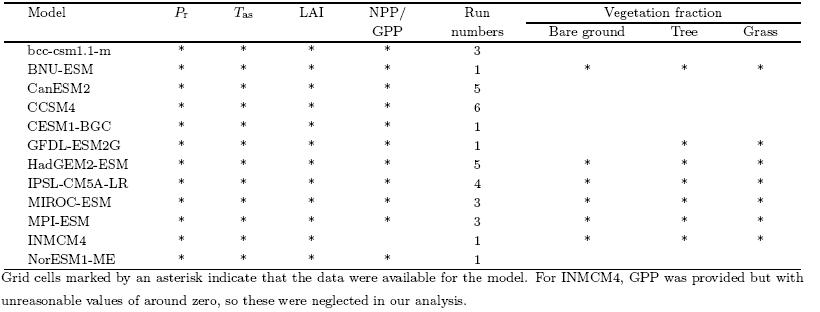
Twelve ESMs with vegetation dynamic distribution(including both DGVM outputs and non-DGVMoutputs)from CMIP5 were selected in this study. Table 1 lists the model names and summarizes the components and characteristics of each ESM. In terms ofthe l and surface, apart from bcc-csm1. 1-m and IN-MCM4, all of the models account for l and use change;likewise, apart from BNU-ESM, NorESM1-ME and CESM1-BGC, none of the models have an interactive l and nitrogen cycle. Several biological variablessuch as LAI, plant functional types(PFTs), net primary productivity(NPP), gross primary productivity(GPP), and the climatic fields related to vegetationgrowth and terrestrial carbon budget such as precipitation(Pr) and surface air temperature(Tas), are provided in the models' outputs. These variables are notavailable for every model, e. g., NPP for INMCM4 isunavailable, GPP for INMCM4 is available but withunrealistic values(most GPP values are around zero), and only 6 of the 12 ESMs provide outputs of PFTs. Table 2 lists the variables used in our analysis(markedby asterisks).
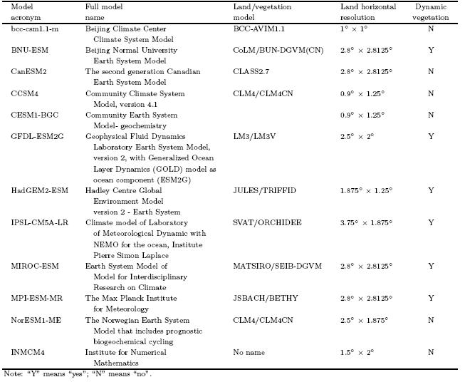
Although the vegetation models in this study differ in their representations of vegetation types, soilproperties, carbon, and nitrogen pools, as well as theirhorizontal and vertical resolutions at the surface and in the atmosphere and ocean, there are some similarities in their treatment of vegetation cover and the terrestrial carbon cycle: plants are categorized into several different PFTs, and the parameterizations for leafphotosynthesis, autotrophic respiration, carbon allocation, and phenology are similar across the models, although their specific parameters and limiting conditions are different. For instance, in most of the ESMs, the leaf carbon pool(Cleaf)is related to LAI via theequation
where SLA is the specific leaf area, which is either aPFT-specific constant or a value that varies along thevertical gradient in the canopy(Thornton and Zimmermann, 2007).
Our analysis focuses on the period 1950-2005(theconcentration-driven historical period)referred to asthe "20th-century simulation" period. The last 20years of this period(1986-2005)form a particular focus due to the reliable and complete observationalrecord during this time, which is suitable for comparison purposes. Although the CMIP5 archive includes daily means for a selection of variables, only themonthly-mean output is used in our analysis, since thistemporal frequency is high enough to provide a reasonably comprehensive picture of model performanceboth in terms of the mean state of the system, thetrend, and its seasonal and interannual variability.
Before performing the evaluation, the model outputs and observations were preprocessed, including theelimination of snow-cover effects by identifying and filtering the snow-mask points in both the model simulations and observations, and regridding them into acommon resolution of 1± ×1±, with only fractional l and in grid cells considered. It should be noted that someof our selected models performed more than one experiment and generated several groups of outputs(seeTable 2). To ensure the reliability of our analysis, allthe data available from the CMIP5 data portal werecollected and integrated into the model ensemble. 2. 2 Validation data
Data from a variety of sources are used in ourmodel evaluation. Table 3 lists the data sources, temporal and spatial resolutions, and regional mean valuesover the TP and st and ard deviations(SD)provided asthe reference uncertainty(the actual data uncertainties are generally larger than the st and ard deviationsprovided here).
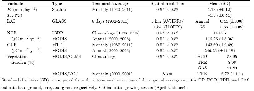
The monthly precipitation(Pr) and surface airtemperature Tas data of 2400 meteorological stationsfrom 1961 to 2010 covering the whole of the Chinesemainl and (Wu and Gao, 2013)are used for the modelevaluation. It is found that precipitation over the TPhas an annual mean value of 1. 13 mm day-1 with anSD of ±0. 12 mm day-1(11%), while surface air temperature has an annual mean of -1. 3 with a largerSD range than precipitation of ±0. 51(39%). 2. 2. 2 LAI, NPP, and GPP
The LAI product of the Global L and Surface Satellite(GLASS)dataset is generated fromthe Advanced Very High Resolution Radiometer(AVHRR)(1982-1999) and the Moderate ResolutionImaging Spectroradiometer(MODIS)reflectance data(2000-2011)using general regression neural networks(GRNNs)(Liang et al., 2013; Xiao et al., 2014). Different from the existing neural network methods that useonly remote sensing data acquired at a specific timeto retrieve LAI, the reprocessed MODIS reflectancedata for an entire year were input into the GRNNsto estimate 1-yr LAI profiles. The MODIS reflectanceproduct(MOD09A1)provides surface reflectance foreach of the MODIS l and spectral b and s with a 500-mspatial resolution and an 8-day temporal sampling period. The AVHRR reflectance data are from NASA'sL and Long Term Data Record(LTDR)project, whichreprocessed Global Area Coverage(GAC)data fromAVHRR sensors onboard NOAA satellites and createda daily surface reflectance product on a 0. 05° spatialresolution. The maximum value composite(MVC)approach is used to composite the daily surface reflectance data into composites of 8-day intervals inorder to maintain a consistent time resolution withMODIS surface reflectance data. The time series of red and near-infrared(NIR)reflectance data of AVHRR and MODIS are used to generate the GLASS LAIproduct. The data quality of the MODIS and AVHRRimages is greatly influenced by clouds, cloud shadows, snow, and other abnormal climate conditions, whichhinder the surface reflectance inversion and further impact the quality of the GLASS products. Some data, such as AVHRR, MOD09A1, MOD09GA, MCD43B3, and MOD02, are preprocessed before being used toproduce the GLASS products. To improve the dataquality, the existing MODIS snow and cloud mask and the reflectance characteristics of the non-snow/cloudpixels are used in combination to identify pixels ofsnow, clouds and abnormal values. All of the identified values are filled by the clear pixel. GLASS LAI onthe TP shows an annual mean of 0. 44 with an SD of±0. 06(13. 6%), and a mean value for the growing season(GS; April-October)of 0. 66 with an SD of ±0. 09(13. 6%).
The International Geosphere Biosphere Programme(IGBP)Global NPP Model IntercomparisonData were used to compare with the simulated NPP. The IGBP NPP data were obtained from the websiteof the International Satellite L and Surface Climatology Project, Initiative II(ISLSCPII)with a resolutionof 0. 5±. The IGBP NPP data were derived from anoriginal dataset containing both the gridded averageNPP values from 17 global models of biogeochemistry(Cramer et al., 1999; Cramer, 2011)for 1986-1995 and their climatological average(http://daac. ornl. gov/cgi-bin/dsviewer. pl?ds-id=1027). This dataset is popularfor model validation(Dan et al., 2007; Fisher et al., 2008), although it is a simulation product. The IGBPNPP data show an annual mean NPP value of 150. 25g C m-2 yr-1 with a wide uncertainty range of 6%-100% according to the o±cially provided SD. To makeour evaluation more precise, the annual mean NPP and GPP data from MODIS(Zhao et al., 2005, 2006, 2010)with a 1-km resolution covering the period 2000-2012 are also used. The data quality is affected by theuncertainties in descriptions of the biome type and meteorological input data, as well as in the algorithm thattranslates measured parameters into inferred processrates. It has also been indicated that these uncertainties may be large in some regions or during certainseasons(Zhao et al., 2005). It is found that MODISNPP and GPP have mean values of 116. 25 and 143. 69g C m-2 yr-1 respectively, with relatively small SDvalues of ±8. 06 g C m-2 yr-1(7%) and ±9. 49 g Cm-2 yr-1(6. 6%), suggesting that the MODIS products are of high quality. The GPP data derived fromthe global upscaling flux tower measurements on theglobal scale based on the model tree ensemble(MTE)approach with the relatively long time series(1982-2012)described by Jung et al. (2009, 2011)are alsoused for the validation. Jung et al. (2011)estimatedthe uncertainty of globally averaged GPP to be ±6 kgC m-2 yr-1(< 15%). In the TP region, the GPP datashow an annual mean value of 246. 25 g C m-2 yr-1, with a small and ideal SD range of ±14. 18 g C m-2yr-1(5. 8%). 2. 2. 3 Vegetation cover
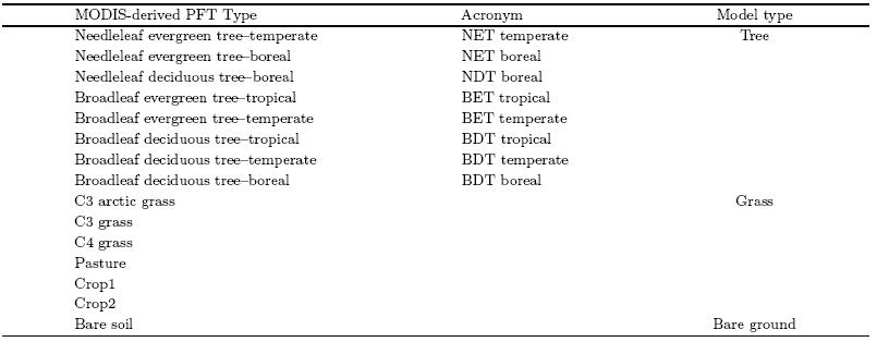
The Community L and Model version 4(CLM4)vegetation fraction data(Lawrence et al., 2007, 2011)derived from MODIS(hereafter MODIS/CLM4), which cover the whole global l and surface with a highresolution of 0. 5° × 0. 5°, are used to evaluate the fractional distributions of bare ground and two vegetationcover types: trees and grass. The MODIS Vegetation Continuous Fields(VCF)dataset for vegetationcover(hereafter MODIS/VCF)derived from Hansenet al. (2003)is also used for evaluation of tree and bareground simulations in this study. These two datasetsdescribe the l and surface in fractions of vegetationcover types: woody vegetation(trees and shrubs), herbaceous vegetation(grasses and crops), and bare(non-vegetated)ground. This is similar to the wayin which DGVMs describe the vegetation cover(orPFTs), which is why they are chosen for our evaluation. For comparison, the MODIS-derived and model-simulated PFTs are placed into three broad vegetationclasses: bare ground, tree, and grass PFTs. Table 4 provides the details of these classifications. The treefraction of MODIS/VCF shows a mean value of 6. 72%with an uncertainty of 1. 1%(14. 8%). Note that inmost of the ESMs, the anthropogenic l and use is predetermined; in particular, the extent of pasture and cropl and is prescribed, and the dynamic vegetationmodels used only affect the natural vegetation distribution. Therefore, only the evaluation of the coverageof natural vegetation is performed here, and the l and cover variation due to transitions from natural to anthropogenic vegetation, and vice versa, is not considered.
A series of analyses were conducted for evaluating and ranking the models. In the following, we describethe diagnostics used for model evaluation and the metrics used for model ranking. 2. 3. 1 Evaluation metrics
There are multiple metrics that can be used forevaluating the agreement between simulated and observed LAI and vegetation cover. Here, the squareof the Pearson correlation coe±cient(r2)is used toquantify the spatial correlation between the vegetation distribution in the model and observation. In alinear approximation, this metric quantifies a fractionof variation explained by the model as
where Mi and Oi are the variables simulated by themodel or observed in the grid cell i, and Wi is an arealweight of grid cell i(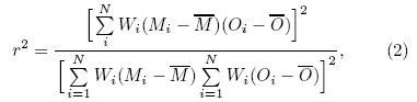
 ). Here, we calculatedWi in the Pearson correlation coe±cient(CC)equa-tion based on the area of each grid associated with thecentral geographic latitude of each grid. In our case, the study region(i. e., the TP)covers 25°-40°N, wherethe values of Wi do not vary much and can almost beneglected. N is the total number of grid cells underevaluation.
The amplitude of the difference between twodatasets is measured by using the root-mean-squareerror(RMSE):
The two metrics, r2 and RMSE, are calculated sepa-rately for LAI and each vegetation class. During thisprocess, the model is evaluated at every grid point and then aggregated over the entire l and surface of the TP. 2. 3. 2 Ranking metrics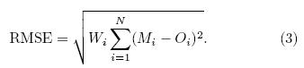
The method described in Section 2. 3. 1 cannotfully identify the best and the worst models among the12 ESMs with respect to TP vegetation simulation. Accordingly, a ranking method is used to assess themodel performance with three ranking metrics. Onemetric is an upgraded version of Eq. (3), with theaim to check the annual seasonal cycle(in terms ofmonthly data)of vegetation features:
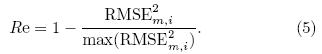
where t corresponds to the temporal dimension, and N is the number of months. Equation(4)can be nor-malized by the maximum to obtain the relative error(Re)as follows:The other metric, the model variability index(MVI), as introduced by Gleckler et al. (2008) and Scherrer(2011), designed to check the model's representation of the interannual features of the observation, isequated by the ratio of the st and ard deviation of themodel means divided by the st and ard deviation of theobserved means(see Eq. (6)), where σo;i and σm;iare the st and ard deviations of the annual time seriesof the model and observation for a given variable ateach grid cell i, respectively. Perfect model-referenceagreement would result in an MVI value approachingzero. This approach avoids the cancellation effects ofa model when experiencing problems related to excessively large or small interannual variability(IAV)(Gleckler et al., 2008; Scherrer, 2011). It is a goodmethod for assessing the difference between a singlemodel and observation, providing a consistent st and ard for identifying the st and ard deviation of a singlemodel. In some model evaluation studies, an MVI value equalto 0. 5 is considered as a good representation of IAV(Scherrer, 2011; Anav et al., 2013b). However, theMVI threshold can vary markedly, changing in a widerange due to differences in physical variables and studyregions, especially biological variables. For example, Anav et al. (2013b)showed that, on the global scale, calculated MVI of LAI and GPP from 18 models ofCMIP5 had ranges of 2-6 and 1-10, respectively, and the ranges were even wider in the Southern Hemisphere. Previous studies have shown that numericalmodels generally perform poorly over the TP than inother places of China due to the TP snow coverage, which may have caused large uncertainty. In this case, a much higher and more variable MVI is expected. Tosolve this problem, we normalize the MVI by the maximum to obtain the relative MVI(RMVI)(Eq. (7)). A value approaching 1 is considered to denote the bestlevel of agreement between model and observation. It should be noted that normalizing the skill score cal-culations in this way only yields a measure of how gooda given model is with respect to a particular referencedataset, and does not have any real meaning.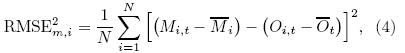

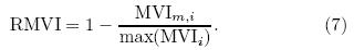
In addition, the bias between a given model(M) and the reference data(O)is also computed as thethird skill score to check the main bias between ESMsimulations and the observation(Eq. (8)). Bm
Similar to the other metrics, models are evaluated atevery grid point and then aggregated over the entirel and area of the TP. 3. CMIP5 model performance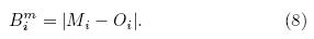
LAI is defined as one side of the green leaf areaper unit ground area in broad leaf canopies and as onehalf of the total needle surface area per unit groundarea in coniferous canopies(Watson, 1947). It is animportant indicator of vegetation state because it affects the radiative transfer process within the canopy, as well as evapotranspiration from the surface, and consequently modulates near-surface climate and atmospheric circulations(Kang et al., 2007). The meanvalues of vegetation distribution are useful for simply quantifying vegetation ecosystem|climate interactions, which may provide insight into model performance, as emphasized in some model intercomparisonstudies. Therefore, we begin by providing general information on the LAI simulations of the 12 ESMs.
Figure 1a shows the simulated LAI compared withthe observed LAI derived from satellite data(GLASS). Large differences are found among the models. Apartfrom CanESM2 and INMCM4, the LAI in the growing season over 1986-2005 in the remaining 10 models is overestimated, with values scattered around theCMIP5 ensemble mean and ranging from 0. 44 to 3. 6. Unrealistically high LAI is found in BNU-ESM and GFDL-ESM2G, with average values greater than 3. 0over the TP. This result is consistent with previousLAI evaluation on the global scale(Anav et al., 2013b;Shao et al., 2013). The overestimation in BNU-ESMis universal around the globe, and the overestimationin GFDL-ESM2G may be caused by a flaw in the l and surface model physics, which allows only coniferoustrees to grow in cold climate in case large LAI contributed by coniferous trees establishes in areas wherethere should be tundra or cold deciduous trees(Anav et al., 2013a). CanESM2 shows a very small boxrange(or slight difference between minimum and maximum), suggesting weak interannual variability in theCanESM2 simulation.
 |
| Fig. 1. Model statistics of LAI in the growing season(April{October), annual mean net primary productivity(NPP), precipitation(Pr), surface air temperature(Tas), and gross primary productivity(GPP). (a)LAI in the growing seasonover the reference period of 1986{2005;(b)annual mean NPP during 1986{1995;(c)NPP during 2000{2005;(d)Pr;(e)Tas;(f)GPP during 1986-1995; and (g)GPP during 2000{2005. Values from top to bottom of each box inside eachpanel are the maximum, 75 percentile, median, 25 percentile, and minimum of the model values during the evaluationperiod. The x-axis identifies the 12 models and the observation dataset. The box values of "ALL" are calculated basedon the model sequences. Each box is marked(*)with the mean value of the individual model. The width of each boxindicates the run numbers for every ESM. In(b, c) and (f, g), NPP and GPP for INMCM4 are missing because they wereunavailable in the CMIP5 data portal. The black lines in each of the panels indicate the mean value of observations. |
For vegetation carbon flux above the ground(orNPP above the ground)during 1986-1995, Fig. 1bshows much more scattered distributions, with magnitudes varying from 125. 8 to 554. 86 g C m-2 yr-1, implying large uncertainty among the models. Withthe exception of CanESM2 and NorESM1-ME, 9 ofthe 11 models(Note that the NPP of INMCM4 wasnot available in the CMIP5 data portal)tend to overestimate the IGBP NPP magnitudes(150. 25 g C m-2yr-1). The systematic bias in NPP generally reflects the accuracy of the simulated LAI shown in Fig. 1a. Following the erroneous pattern of LAI, GFDL-ESM2G, and CanESM2 respectively show the largest and least bias, when compared with the IGBP NPP. For CCSM4 and CESM1-BGC that use CLM4 extended with a carbon-nitrogen(CN)biogeochemicalmodel(hereafter CLM4CN)as their vegetation model, very similar overestimated NPP is simulated. However, NorESM1-ME, which also uses CLM4/CLM4CNas its l and surface/vegetation model but forced bythe revised Community Atmosphere Model version 4(CAM4)(Neale et al., 2010)with CCSM4, an abnormally low NPP mean value is found, suggesting thatthe relationship between LAI and biomass productionin this model is unrealistic. NPP derived from MODISduring 2000-2005 shows a much lower annual meanvalue(116. 25 g C m-2 yr-1)than the IGBP NPPmean during this period, which is severely overestimated by all of the 11 ESMs, and with a much largerrange from 131. 29 to 588. 68 g C m-2 yr-1|even forCanESM2, which is one of the two ESM models thatunderestimate the observed LAI, as mentioned above. The simulated NPP during 2000-2005 shows a 4. 2-65. 3 g C m-2 yr-1 increase with a generally smallerinterannual variability(see the much narrower boxrange)compared with that during 1986-1995, whichis reasonable and consistent with the LAI variations.
The overestimation of LAI may be associatedwith an overestimation of observed precipitation. Itis found that the erroneous pattern of simulated LAIconforms well with the simulated precipitation(Fig. 1d), with the exception of IPSL-CM5A-LR, GFDL-ESM2G, and INMCM4. The large bias found in BNU-ESM could be in some way due to the serious wet biasthat this model has in reproducing the observed precipitation. The mean annual precipitation as reportedby the station data is 1. 12 mm day-1, while BNU-ESM produces a value about 4 times as large(4. 03 mmday-1). CanESM2 shows a small and underestimatedLAI, which is consistent with the relatively small wetbias in the model. The simulated surface air temperature does not contribute much to the overestimatedLAI, since all the models apart from BNU-ESM generate a colder than observed atmosphere near the surfaceof the TP, which is not conducive for plant growth, vegetation photosynthesis, and carbon exchange between vegetation and the atmosphere.
GPP represents the uptake of atmospheric CO2during photosynthesis. Anav et al. (2013b)attributedthe overestimated LAI in 18 ESM models from CMIP5to two reasons. One is associated with the overestimated photosynthesis(or GPP), which could lead toa surplus of biomass stored into the leaves, and themissing parameterization of ozone also partially explains the LAI overestimation due to the high GPP, with the proof that ozone leads to a mean global LAIreduction of about 10%-20% during the historical period as compared with a simulation without elevatedtropospheric ozone(Sitch et al., 2007; Wittig et al., 2009). In our case, the 12 ESMs are found to seriously overestimate the MODIS(Fig. 1f) and MTE(Fig. 1g)GPP, with a similar erroneous pattern toLAI. Therefore, the overestimation of photosynthesiscould be one of the possible reasons for the LAI overestimation. This highlights the wet bias of models sinceprecipitation is another main limiting factor for plantphotosynthesis across the globe besides temperature. The level of uncertainty in satellite-derived LAI is alsoanother possible reason for the unrealistically overestimated LAI over the TP. This is because remote sensing data cannot represent the real LAI distributionspatially and temporally, although it has been widelyrecognized as a valuable tool for detection and analysis of LAI.
Figure 2 shows spatial distributions of the meanLAI of each model and their ensemble, as well as theGLASS observation in the growing season over thereference period. In general, each model reproducesthe observed LAI pattern, with LAI decreasing fromthe southeast border where forests dominate, to thenorthwestern TP mainly covered by bare l and (Yu et al., 2010). With the exception of CanESM2 and IN-MCM4, LAI in the southeastern TP is severely over-estimated in the remaining models, especially BNU-ESM and GFDL-ESM2G, as mentioned when analyzing Fig. 1a. In addition, CCSM4, CESM1-BGC, and NorESM1-ME produce similar overprediction patterns in southeastern TP due to their use of the samel and /vegetation model. The dark crosses in Fig. 2mark the areas where the simulated interannual variability of LAI is reliably consistent with the observation(p < 0. 05). It can be seen that the simulated interannual variability in most of the models has higherreliability in the eastern and southwestern TP compared to elsewhere. BNU-ESM and GFDL-ESM2Ggenerate increasing LAI in agreement with the observation, albeit with unrealistically high values. However, HadGEM2-ES shows continuously descendingLAI, which is opposite to the observed interannualvariability(figure omitted), implying that there issomething wrong in the vegetation dynamics of theHadGEM2-ES model.
 |
| Fig. 2. Spatial distributions of simulated and observed LAI in the growing season. Figures(a-l) and (m)respectivelyindicate the simulated LAI for the 12 individual models and the model ensemble, while(n)indicates the observed LAI ofGLASS. The hatched areas in(a-m)indicate the grids with statistically significant interannual change(p < 0. 05). Thedark blue lines in each panel are the Yellow River(top) and the Yangtze River(bottom). |
Figure 3 compares the spatial distribution of thelinear trend between the GLASS observation(Figs. 3a-c) and the 12-model ensemble(Figs. 3d-f). Theobservation shows a significant increasing tendency in46% of the area of the TP(p < 0. 05), with the trend< 0. 15 per decade(bar plot in the bottom left)(Figs. 3a and 3b). The most noticeable increase can be seenat the eastern and southern borders, where the coverage is mainly forest(Yu et al., 2010) and where LAI increases by more than 0. 15 per decade(Fig. 3a). However, 2. 2% of the area with the significant decreasingtendency(between -0. 1 and -0. 15 per decade)can alsobe found in the upper reaches(or headstream)of theYellow River and the edges of the northern and western TP, suggesting a degraded vegetation status therein the past 20 years.
 |
| Fig. 3. Spatial distributions of the LAI linear trend, significance level, and consistency during the growing seasonfrom 1986 to 2005 in(a, b, c)the observation and (d, e, f)simulation:(a, d)LAI linear trend(10-3(10 yr)-1);(b, e)significance level of the linear trend, in which the increasing/decreasing significance(p)is expressed quantitatively, with colored areas indicating two divided levels(p < 0. 01 and 0. 01< p < 0. 05);(c)consistency of single models with theobservation(GLASS); and (f)consistency of single models with the model ensemble. Filled colors in(c) and (f)indicatethe cumulative number of models showing a trend(increasing or decreasing)that is consistent with the observation orthe 12-ESM ensemble. The insets show the(a, d)frequency distributions of the corresponding trends, (b, e)di®erentsignificance levels, and (e, f)model numbers greater than 6. |
The model ensemble shows a distinct increasingtrend of LAI, with an exp and ed area of 82% over theTP and a comparable trend of 0. 05-0. 15 per decadein the observation(Figs. 3d and 3e). At the south-ern and eastern borders of the TP, the ensemble sim-ulation shows a slightly small increasing trend(0. 10to -0. 15 per decade)compared with the observation. However, the evident decreasing trend found in theupper reaches of the Yellow River is not clearly shownin the model ensemble due to the low resolution of themodels.
The consistency of the model simulations with theobservation reflects the reliability of the simulationsto a certain degree. It is indicated that the modelscan generally reflect the variation of observed LAI inthe reference period, with 8 of the 12 models illustrating consistent increasing trends with the observationin more than 80% of the area(Fig. 3c). As mentionedabove, the apparent disagreement exists at the northern border and headstream of the Yellow River, wherethe simulated LAI shows a strong increasing trend thatis out of phase with the observation. The model simulations show better agreement with the model ensemble than that with the observation, with approximately 80% of the area possessing a coherent increasing tendency, simulated by more than 10 models.
Figure 4 shows the seasonal evolution of observed and simulated LAI for the entire TP. The GLASS observation indicates a clear interannual cycle, with theLAI magnitude showing a remarkable increase in Maywhen the vegetation of the TP starts to green up, reaching its peak in June and July, before recoveringto a low in the dormancy period after October. Mostmodels show a seasonal cycle with its phase in agreement with the observation, except IPSL-CM5A-LR, which does not present a complete seasonal variationas the other models do, although the start of the growing season is not accurately simulated by the othermodels(e. g., HadGEM-ESM2 shows a one-month advance, and CanESM2 and INMCM4 a one-month delay). For GFDL-ESM2G and BNU-ESM, the simulated LAIs show unrealistically high values for the entire year, even during the dormancy seasons, with theformer possessing a very small seasonal variability and the latter an extremely high LAI(maximum of 4. 4)during summer(June-August). The extensive coverage of evergreen vegetation(trees, shrubs, or tundra) and the seasonal herbaceous vegetation or deciduoustrees, are respectively considered to contribute to theiroverestimated LAI. Our assumption does not conflictwith the previous explanation for overestimated LAIin GFDL-ESM2G, since coniferous trees are also partof the evergreen vegetation. The underestimation ofLAI in CanESM2 is probably related to the delayedstart of the growing season. A similar pattern of seasonal variation is shown in CCSM4, CESM1-BGC, and NorESM1-ME simulations, which stresses the importance of vegetation model performance to simulatedvegetation dynamics.
 |
| Fig. 4. Observed and simulated climatological monthly mean LAI during the reference period 1986-2005 for eachcalendar month. Color intensities reflect the magnitude of the climatological LAI mean. The x-axis corresponds tocalendar months, and the y-axis indicates the 12 ESMs, its ensemble, and the observation(GLASS). |
For vegetation cover, only three classes(bareground, trees, and grass)are focused upon, sincethey have the widest coverage on the TP and thestrongest effect on biophysical properties of the l and surface(Brovkin et al., 2013). Figure 5a shows thearea-averaged PFTs of bare ground, trees, and grassfrom model simulations during 1986-2005 comparedwith the observations of MODIS/CLM4. The modelsgenerally underestimate bare ground(except GFDL-ESM2G) and overestimate tree coverage(except IPSL-CM5A-LR), with very scattered grass coverage, although individual models capture well the observedPFTs(e. g., both HadGEM2-ES and MPI-ESM-LRsimulate comparable coverages of bare ground and trees with the observation).
During the period from the middle of the 20thto the early 21st century, the model ensemble shows aslight increase in bare ground and decrease in tree coverage, with respective trends of 0. 58% and -1. 48% perdecade(Fig. 5b). The simulated grass coverage doesnot show significant variations during this period. Inthe last two decades(1986-2005), the simulated treecoverage shows a continuous but much more moderatedescending trend(-0. 18% per decade), while the bareground area turns to a slight decrease(-0. 08% perdecade); the sign of grass variation is still too weak tobe discerned.
 |
| Fig. 5. Observed and simulated vegetation coverage. (a)Three PFTs over the TP. The tree fraction in HadGEM2-ES and bare ground fraction in MIROC-ESM are not shown since they are within 5%, which is considered to have insu±cientaccuracy. (b)Temporal variation of PFT coverage for the model ensemble over the period 1950-2005. The black dashedlines in(b)indicate the linear trends of the three PFTs, and "rc" indicates the trends of the PFTs. |
Figure 6 shows the MODIS/VCF and simulatedspatial coverage for bare ground(Figs. 6a and 6d), trees(Figs. 6b and 6e), and grass(Figs. 6c and 6f). It can be seen from the observation that bare groundis mainly located in the northwestern TP, and there isalmost no bare ground coverage at the southern and eastern borders(Fig. 6a). Tree coverage exists mainlyat the southeastern edge of the TP, with a high fraction of over 80% in most of the area. In the south-eastern TP, grass is the dominant biome type, with anarea of coverage of 40. 82%.
 |
| Fig. 6. Spatial distributions of(a, b, c)observed and (d, e, f)simulated vegetation coverage(%)during 2000{2001 for(a, d)bare ground, (b, e)trees, and (c, f)grass. |
The simulated distribution of bare ground fromextending tree b and at the northern edge of the TP(Fig. 3e)due to the overestimation of GFDL-ESM2Gas described in Section 3. 2. The observed grass fraction is not captured well by the model ensemble. Unlike the observed grass fraction, which is mainly located in the southeastern TP, the simulated grass fraction from the model ensemble evenly covers the entireTP, with a PFT fraction two times of that of the observation.
It is clear that CMIP5 ESMs cannot well reproduce the observed PFTs. Besides the systemic biasof PFTs in the models, the large differences betweenCMIP5 ESM outputs and observations may also bedue to the ESMs' coarse spatial resolutions, whichdoes not adequately represent the control that thecomplex topography has on the vegetation distribution of the TP, even when they are downscaled to arelatively high resolution of 1° × 1° as in our analysis. As a result, the heterogeneous spatial distributions of surface air temperature and precipitation aresmoothed compared to observations, which then influence the resulting vegetation distribution.
To facilitate comparisons in a concise way, thesquare of the Pearson correlation coe±cient(r2) and the root-mean-square error(RMSE), as well as a Taylor diagram, are used to quantify the performance ofthe model simulations. Table 5 lists the values of r2 and RMSE separately for LAI and the three PFTsmentioned above. Over the TP, r2 and RMSE of LAIare equal to 0. 69 and 1. 25, respectively, which are comparable with the result of Brovkin et al. (2013)basedon CMIP5 ESM simulations on the global scale. Themodel ensemble shows a relatively higher r2 and lowerRMSE values(0. 59 and 14. 48%)for tree fraction, whencompared with bare ground and grass. The grass fraction, as an intermediate class between tree and bareground coverage, is reproduced less reliably over theTP, with r2 of 0. 19 and RMSE of 31. 61%.
Figure 7 shows the Taylor diagram(Taylor, 2001)derived from the st and ard deviations and correlationcoe±cients of LAI in the growing season. The distancefrom point to point(1. 00, 1. 00)in the Taylor diagramindicates the relative skill of the model. It can be seenthat the normalized st and ard deviations spread outover a large range from 0. 75 to 2. 79. Most of the models show larger interannual variability than the observation, with the ratio of the st and ard deviation to theobservation being more than 1, except for CanESM2 and MPI-ESM-LR, which also have smaller relativebias(< 50%)than other models, suggesting that thesemodels perform well in reproducing the observed meanstate. Of the 12 models, INMCM4 shows the closestvalue with the observation, while NorESM1-ME showsthe most dispersed st and ard deviation from the observation.
The correlation coe±cients reflect agreement between the model simulations and the observation interms of spatial distribution. It is shown in Fig. 7 that the correlation coe±cient values spread wit-hin the range of 0. 65-0. 90, with most models having ahigh value of more than 0. 8, except HadGEM2-ES and MIROC-ESM. Models CCSM4, CESM1-BGC, and NorESM1-M show relatively high correlation coefficient values of 0. 89 in their simulations. This suggestsgood ability of CLM4/CLM4CN to represent observedspatial distributions of LAI.
 |
| Fig. 7. Taylor diagram of LAI during the growing seasonfor the reference period(1986-2005). The correlations and ratios of st and ard deviations among model simulations and the observation(GLASS)are calculated spatially. |
The diagnostics in Section 3 indicate that, generally, the CMIP5 ESMs can adequately reproducethe observed biological characteristics of vegetation, although a few of the models do show notably pooreragreement than others, and general problems exist forquite a few of the models. The measures provide thebasic information of model performance, which is crucial for identifying model differences in a model evaluation system. However, the diagnostics are not sufficient to clearly identify the best and worst modelsin model ensemble members. To achieve this objective, specific metrics were defined(see Eqs. (4)-(8)) and calculated to produce a quantitative ranking ofthe models.
Figure 8 shows the skill scores of simulated LAIin terms of the metrics defined in Eqs. (4)-(8). Itis indicated that CanESM2, MPI-ESM-LR, and IN-MCM4 posses the best skills for reproducing observedamplitude and seasonal evolution(see "Re" of Figs. 8a and 1a), although it seems to be two months out ofphase with the observation during the peak season forCanESM2(Fig. 4). The poorest performance is foundin BUN-ESM and NorESM1-ME, mainly due to theirgreat discrepancies in LAI magnitude with the observation of GLASS(Fig. 1a). The relatively low skillscore for IPSL-CM5A-LR(ranking number of 7)is related to its bad representation of seasonal evolution, since the simulation is totally out of phase comparedwith the observation(Fig. 4). Our results are consistent with another study based on CMIP5 biologicalvariables on the global scale(Anav et al., 2013b).
The models show very different skill scores whenranked with respect to interannual variability, e. g., bcc-csm1. 1-m and MPI-ESM-LR achieve the top twoscores among all 12 models(see "RMVI" in Fig. 8a). The simulations of CCSM4, CESM1-BGC, as well asNorESM1-ME, all achieve high scores, indicating goodability of CLM4 to represent interannual variability. Among the 12 models, CanESM2 and GFDL-ESMshow the worst simulation skills in reproducing interannual variability of LAI.
 |
| Fig. 8. Model ranking with respect to LAI:(a)modelranking results based on relative error(Re)calculated byEqs. (4) and (5) and relative model variability index(RMVI)calculated by Eqs. (6) and (7);(b)model rankingresult based on absolute bias(BIAS)between simulations and the observation calculated by Eq. (8). |
Figure 8b shows an absolute measure of theESMs' skills in reproducing the mean state of observed LAI. As in Figs. 1a and 7, CanESM2 and IN-MCM4 present the smallest bias of the 12 ESMs, whencompared with the observed LAI. It is not surprisingthat GFDL-ESM and BNU-ESM show very poor skill, which in both cases is related to the improper description of l and surface model physics and the large wetbias, as previously mentioned.
Finally, we calculated the arithmetic product ofweights according to the ranking orders for Re, RMVI, and BIAS, with the ranking number greater than 10(here larger numbers mean poorer simulation skill)outof the lists, and then obtained the ranking sequence forthe model group. It was found that INMCM4, bcccsm1-m, MPI-ESM-LR, IPSL-CM5A-LR, HadGEM2ES, and CCSM4 perform the best among the 12 models. No model ranking was performed for vegetation cover due to the deficiency of monthly vegetationcover. It is important to note that the model rankingresults are dependent on the selection of variables and skill score metrics applied, as well as the study region. Therefore, this result is limited to the conditions ofthe present analysis only. 5. Conclusions and discussion
In this study, the abilities of 12 CMIP5 ESMs toreproduce the mean state, trends, seasonal cycle, and interannual variability of vegetation dynamics for thepresent day over the TP have been evaluated by comparing against the remotely sensed biological vegetation products. Several metrics, including three ranking metrics, were applied to identify the strengths and weaknesses of the individual models, as well as theirsystematic biases.
The LAI patterns generated by the models agreewell with the observed data, though most of the models tend to overestimate the satellite LAI magnitude, with r2 and RMSE values of 0. 69 and 1. 25 respectivelyfor the model ensemble. The simulated NPP is generally overestimated when compared with the IGBPNPP(except for CanESM2 and NorESM1-ME) and MODIS NPP during different periods. The wet biasfound in most models and overestimation of photosyn-thesis as well as the bias of satellite data, are considered to be plausible reasons for the overestimation ofsimulated LAI in most of the models. The model simulations capture the observed increasing trend of LAIover most of the TP during the period 1986-2005; however, the decreasing trend around the headstream ofthe Yellow River is not detected due to the coarse resolution of the ESMs. The model ensemble producesoverestimated bare ground and underestimated treefraction, with r2 values of 0. 56 and 0. 59 for bare soil and tree fraction respectively. Grass coverage showsthe poorest performance. During 1950-2005, bareground over the TP shows a slight increasing trend of0. 58% per decade, while forest is decreasing at 1. 48%per decade. Grass coverage does not show any significant variation. The models show very different skillscores in their simulations of the seasonal evolution and interannual variability. By synthetically considering the model performance in terms of the meanstate, seasonal and interannual variability comparedwith observed LAI, INMCM4, bcc-csm1-1m, MPI-ESM-LR, IPSL-ESM-LR, HadGEM2-ES, and CCSM4are ranked the best models in representing the vegetation characteristics of the TP.
In our study, LAI and vegetation cover have beenevaluated by using two metrics(r2 and RMSE)toshow the general performance of model simulations, and we carried out vegetation cover validation separately on three classes. There are a number of othermetrics used for vegetation biophysical variables. Forexample, Monserud and Leemans(1992)used j statistics to evaluate discrete vegetation, Poulter et al. (2011)attempted to evaluate vegetation cover simultaneously in more than two classes based on the b-diversity metric(mean Euclidean distance). The chosen metrics depend mainly on the research objective. Similarly, the relatively simple skill score metrics ofRe, RMVI, and BIAS were adopted for the modelranking in this study, but there are more complicated and mature metrics(Brunke et al., 2003; Decker et al., 2012; Wang and Zeng, 2012)that could also be usedfor ranking the models.
The CCSM4, CESM1-BGC, and NorESM1-ME, which share CLM4/CLM4CN as their l and surfacemodel and vegetation model, show some commonweaknesses and strengths in their simulations, such asgood performance in representing the observed spatial distribution, seasonal cycle, and interannual variability, and bad performance in reproducing the meanvalues of observed LAI and NPP. This suggests the importance of l and surface and vegetation physics for thesuccessful description of vegetation dynamics. It wasalso noted in our analysis that the simulated PFT fractions show much poorer performance compared withLAI, for both the mean state and the spatial distribution, which highlights a major weakness for modeldevelopers to work on for future model improvements.
Acknowledgments:We thank the Beijing Normal University for providing the Global Products ofEssential L and Variables(GLASS). Dr. ZhaoMaosheng, Martin Jung, and Victoria Brovkin arethanked for providing the MODIS NPP, GPP, modeltree ensembles(MTE)GPP and MODIS/VCF vegetation cover datasets. We thank Dr. Gao Xuejiefor providing the 2400 meteorological station dataof China. The two anonymous reviewers are alsothanked for their insightful comments and suggestions, which helped to improve the quality of themanuscript. We acknowledge the computing resources and time of the Supercomputing Center of Cold and Arid Regions Environment and Engineering ResearchInstitute of the Chinese Academy of Sciences. Wealso acknowledge the modeling groups from BCC, BNU, CCCma, GFDL, INM, IPSL, MIROC, MOHC, MPI-M, NCAR, and NCC, and the World ClimateResearch Programme's(WCRP)Working Group onCoupled Modeling(WGCM)for making the modeloutput available on the U. S. Department of EnergyPCMDI server.
| [1] | Abramowitz, G., R. Leuning, M. Clark, et al., 2008: Evaluating the performance of land surface models. J. Climate, 21, 5468-5481. |
| [2] | Anav, A., G. Murray-Tortarolo, P. Friedlingstein, et al., 2013a: Evaluation of land surface models in reproducing satellite derived leaf area index over the high-latitude Northern Hemisphere. Part II: Earth system models. Remote Sens., 5, 3637-3661. |
| [3] | —-, P. Friedlingstein, M. Kidston, et al., 2013b: Evaluating the land and ocean components of the global carbon cycle in the CMIP5 Earth System Models. J. Climate, 26, 6801-6843. |
| [4] | Arneth, A., S. P. Harrison, S. Zaehle, et al., 2010: Terrestrial biogeochemical feedbacks in the climate system. Nature Geosci., 3, 525-532. |
| [5] | Bathiany, S., M. Claussen, V. Brovkin, et al., 2010: Combined biogeophysical and biogeochemical effects of large-scale forest cover changes in the MPI earth system model. Biogeosci. Discuss., 7, 1383-1399. |
| [6] | Blyth, E., D. Clark, R. Ellis, et al., 2011: A comprehensive set of benchmark tests for a land surface model of simultaneous fluxes of water and carbon at both the global and seasonal scale. Geosci. Model Dev., 4, 255-269. |
| [7] | Brovkin, V., L. Boysen, T. Raddatz, et al., 2013: Eval-uation of vegetation cover and land-surface albedo in MPI-ESM CMIP5 simulations. J. Adv. Modeling Earth Syst., 5, 48-57. |
| [8] | Brunke, M. A., C. W. Fairall, X. B. Zeng, et al., 2003: Which bulk aerodynamic algorithms are least prob-lematic in computing ocean surface turbulent fluxes? J. Climate, 16, 619-635. |
| [9] | Cadule, P., P. Friedlingstein, L. Bopp, et al., 2010: Bench-marking coupled climate-carbon models against long-term atmospheric CO2 measurements. Global Biogeochem. Cy., 24, doi: 10.1029/2009GB003556. |
| [10] | Collins, W., N. Bellouin, M. Doutriaux-Boucher, et al., 2011: Development and evaluation of an earth-system model—HadGEM2. Geosci. Model Dev. Discuss., 4, 997-1062. |
| [11] | Cramer, W., 2011: ISLSCP II IGBP NPP output from terrestrial biogeochemistry models. ISLSCP Initia-tive II Collection. Data Set. Hall, F. G., G. Collatz, B. Meeson, et al., Eds., Oak Ridge National Labo-ratory Distributed Active Center, Oak Ridge, Ten-nessee, U. S. A., doi: 10.3334/ORNLDAAC/1027. |
| [12] | —-, D. W. Kicklighter, A. Bondeau, et al., 1999: Comparing global models of terrestrial net primary productivity (NPP): Overview and key results. Global Change Biology, 5(S1), doi: 10.1046/j.1365-2486.1999.00009.x. |
| [13] | Dan, L., J. J. Ji, and Y. He, 2007: Use of ISLSCP II data to intercompare and validate the terrestrial net pri-mary production in a land surface model coupled to a general circulation model. J. Geophys. Res. Atmos. (1984-2012), 112, doi: 10.1029/2006JD007721. |
| [14] | Decker, M., M. A. Brunke, Z. Wang, et al., 2012: Evalu-ation of the reanalysis products from GSFC, NCEP, and ECMWF using flux tower observations. J. Climate, 25, 1916-1944. |
| [15] | Fisher, J. B., K. P. Tu, and D. D. Baldocchi, 2008: Global estimates of the land-atmosphere water flux based on monthly AVHRR and ISLSCP-II data, validated at 16 FLUXNET sites. Remote Sens. Environ., 112, 901-919. |
| [16] | Gleckler, P. J., K. E. Taylor, and C. Doutriaux, 2008: Performance metrics for climate models. J. Geo-phys. Res. Atmos. (1984-2012), 113, doi: 10.1029/2007JD008972. |
| [17] | Hansen, M. C., R. S. DeFries, J. R. G. Townshend, et al., 2003: Global percent tree cover at a spatial res-olution of 500 meters: First results of the MODIS vegetation continuous fields algorithm. Earth Inter-act., 7, 1-15. |
| [18] | IPCC, 2007: Summary for Policymakers. Climate Change 2007: The Physical Science Basis. Contribution of Working Group I to the Fourth Assessment Report of the Intergovernmental Panel on Climate Change. Solomon, S., et al., Eds., Cambridge University Press, 996 pp. |
| [19] | Jung, M., M. Reichstein, and A. Bondeau, 2009: Towards global empirical upscaling of FLUXNET eddy co-variance observations: Validation of a model tree ensemble approach using a biosphere model. Bio-geosci., 6, 2001-2013. |
| [20] | —-, —-, H. A. Margolis, et al., 2011: Global patterns of land-atmosphere fluxes of carbon dioxide, latent heat, and sensible heat derived from eddy covari-ance, satellite, and meteorological observations. J. Geophys. Res. Biogeosci. (2005-2012), 116, doi: 10.1029/2010JG001566. |
| [21] | Kang, H.-S., Y. K. Xue, and G. J. Collatz, 2007: Im-pact assessment of satellite-derived leaf area index datasets using a general circulation model. J. Climate, 20, 993-1015. |
| [22] | Kato, T., Y. H. Tang, S. Gu, et al., 2004: Carbon diox-ide exchange between the atmosphere and an alpine meadow ecosystem on the Qinghai-Tibetan Plateau, China. Agric. Forest Meteor., 124, 121-134. |
| [23] | Lawrence, D. M., K. W. Oleson, M. G. Flanner, et al., 2011: Parameterization improvements and func-tional and structural advances in version 4 of the Community Land Model. J. Adv. Modeling Earth Syst., 3, doi: 10.1029/2011MS00045. |
| [24] | Lawrence, P. J., and T. N. Chase, 2007: Represent-ing a new MODIS consistent land surface in the Community Land Model (CLM 3. 0). J. Geo-phys. Res. Biogeosci. (2005-2012). 112, doi: 10.1029/2006JG000168. |
| [25] | Liang, S. L., X. Zhao, S. H. Liu, et al., 2013: A long-term global land surface satellite (GLASS) dataset for en-vironmental studies. Int. J. Digital Earth, 6(Sup1), 5-33. |
| [26] | Monserud, R. A., and R. Leemans, 1992: Comparing global vegetation maps with the Kappa statistic. Ecological Modeling, 62, 275-293. |
| [27] | Neale, R. B., C. Chen, A. Gettelman, et al., 2010: De-scription of the NCAR Community Atmosphere Model (CAM 5. 0). NCAR Tech. Note NCAR/TN-486+STR. 274 pp. |
| [27] | Piao, S. L., J. Y. Fang, and J. S. He, 2006: Variations in vegetation net primary production in the Qinghai-Xizang Plateau, China, from 1982 to 1999. Climatic Change, 74, 253-267. |
| [28] | —-, —-, P. Ciais, et al., 2009: The carbon balance of terrestrial ecosystems in China. Nature, 458, 1009-1013. |
| [29] | —-, P. Ciais, Y. Huang, et al., 2010: The impacts of climate change on water resources and agriculture in China. Nature, 467, 43-51. |
| [30] | Port, U., V. Brovkin, and M. Claussen, 2012: The role of dynamic vegetation cover in future climate change. Earth Syst. Dyn. Discuss., 3, 485-522. |
| [31] | Poulter, B., P. Ciais, E. Hodson, et al., 2011: Plant functional type mapping for earth system models. Geosci. Model Dev. Discuss., 4, 2081-2121. |
| [32] | Randerson, J. T., F. M. Hoffman, P. E. Thornton, et al., 2009: Systematic assessment of terrestrial biogeo-chemistry in coupled climate-carbon models. Global Change Biology, 15, 2462-2484. |
| [33] | Scherrer, S. C., 2011: Present-day interannual variability of surface climate in CMIP3 models and its relation to future warming. Int. J. Climatol., 31, 1518-1529. |
| [34] | Shao, P., X. P. Zeng, K. Sakaguchi, et al., 2013: Terrestrial carbon cycle: Climate relations in eight CMIP5 earth system models. J. Climate, 26, 8744-8764. |
| [35] | Sitch, S., P. M. Cox, W. J. Collins, et al., 2007: Indirect radiative forcing of climate change through ozone ef-fects on the land-carbon sink. Nature, 448, 791-794. |
| [36] | Tan, K., P. Ciais, S. Piao, et al., 2010: Application of the ORCHIDEE global vegetation model to eval-uate biomass and soil carbon stocks of Qinghai-Tibetan grasslands. Global Biogeochem. Cy., 24, doi: 10.1029/2009GB003530. |
| [37] | Taylor, K. E., 2001: Summarizing multiple aspects of model performance in a single diagram. J. Geophys. Res. Atmos. (1984-2012), 106, 7183-7192. |
| [38] | Thornton, P. E., and N. E. Zimmermann, 2007: An im-proved canopy integration scheme for a land surface model with prognostic canopy structure. J. Climate, 20, 3902-3923. |
| [39] | Wang, A. H., and X. B. Zeng, 2012: Evaluation of mul-tireanalysis products with in situ observations over the Tibetan Plateau. J. Geophys. Res. Atmos. (1984-2012), 117, doi: 10.1029/2011JD016553. |
| [40] | Watanabe, S., T. Hajima, K. Sudo, et al., 2011: MIROC-ESM: Model description and basic results of CMIP5-20c3m experiments. Geosci. Model Dev. Discuss., 4, 1063-1128. |
| [41] | Watson, D. J., 1947: Comparative physiological studies on the growth of field crops. I: Variation in net assimilation rate and leaf area between species and varieties, and within and between years. Ann. Bot., 11, 41-76. |
| [42] | Wittig, V. E., E. A. Ainsworth, S. L. Naidu, et al., 2009: Quantifying the impact of current and future tropo-spheric ozone on tree biomass, growth, physiology and biochemistry: A quantitative meta-analysis. Global Change Biology, 15, 396-424. |
| [42] | Wu Jia and Gao Xuejie, 2013: A gridded daily observa-tion dataset over China region and comparison with the other datasets. Chinese Geophys., 56, 1102-1111. (in Chinese) |
| [43] | Xiao, Z. Q., S. L. Liang, J. D. Wang, et al., 2014: Use of general regression neural networks for generating the GLASS leaf area index product from time-series MODIS surface reflectance. Geosci. Remote Sens., 52, 209-223, doi: 10.1109/TGRS.2013.2237780. |
| [44] | Yu, H., E. Luedeling, J. Xu, 2010: Winter and spring warming result in delayed spring phenology on the Tibetan Plateau. Proc. Natl. Acad. Sci. USA, 107, 22151-22156. |
| [45] | Zhang, P., M. Hirota, H. Shen, et al., 2009: Characteriza-tion of CO2 flux in three Kobresia meadows differing in dominant species. J. Plant Ecol., 2, 187-196. |
| [46] | Zhao, M. S., F. A. Heinsch, R. R. Nemani, et al., 2005: Improvements of the MODIS terrestrial gross and net primary production global data set. Remote Sens. Environ., 95, 164-176. |
| [47] | —-, S. W. Running, and R. R. Nemani, 2006: Sensi-tivity of Moderate Resolution Imaging Spectrora-diometer (MODIS) terrestrial primary production to the accuracy of meteorological reanalyses. J. Geophys. Res. Biogeosci. (2005-2012), 111, doi: 10.1029/2004JG000004. |
| [48] | —-, and S. W. Running, 2010: Drought-induced reduction in global terrestrial net primary production from 2000 through 2009. Science, 329, 940-943. |