 2014, Vol. 28
The Chinese Meteorological Society
Article Information
- ZHANG Chi, LI Qi. 2014.
- Tracking the Moisture Sources of an Extreme Precipitation Event in Shandong, China in July 2007:A Computational Analysis
- J. Meteor. Res., 28(4): 634-644
- http://dx.doi.org/10.1007/s13351-014-3084-9
Article History
- Received December 17, 2013;
- in final form June 5, 2014


1. Introduction
Research into the moisture sources of precipitation is important for underst and ing water cycling(Ralph et al., 2006). Such research reveals the mechanisms by which water is ev aporated from one area, transported, and falls in another area as precipitation. This process is termed moisture recycling or precipitation recycling. There are four categories of moisture recycling models: bulk models, general circulation models(GCMs)with tagged water, Lagrangianmethods, and isotopic analysis.
GCM with tagged water is a tagging techniquein the Eulerian frame. GCMs implement the numerical water vapor tracers(WVTs)that experience thesame processes as atmospheric water(Bosilovich and Schubert, 2002; Gimeno et al., 2012). The ev aporation, transportation, and sink destination of WVTsare tracked and recorded. GCMs may be the mostcomprehensive and complex models in atmosphericscience; they provide the most physical meaning and require the most complex computation. The accuracyof GCMs depends on the simulation or parameterization of various atmospheric processes, such as convection, turbulence, and longwave and shortwave radiation.
The Lagrangian-type methods are divided intotwo kinds. One is the back-trajectory method, whichconsiders water vapor as a passive tracer along quasiisentropic surfaces(Dirmeyer and Brubaker, 1999; Dirmeyer and Brubaker, 2007). This method doeshave some limitations. Kurita et al. (2004)noted thatthe adiabatic assumption of this method may not bevalid in summer over l and . Moreover, precipitation isdivided into many parcels of the same mass that originate from an atmospheric level according to a probability distribution model, which may not be realistic(Fitzmaurice, 2007). The other kind of Lagrangianmethods is based on atmospheric particle dispersion models, which have been incorporated into toolssuch as FLEXP AR T(FLEXible P AR Ticle dispersionmodel; Stohl et al., 2005) and HYSPLIT(HYbrid Single Particle Lagrangian Integrated T ra jectory Model; Draxler and Hess, 1998). The atmospheric particledispersion models also have limitations. They can onlyaccount for the net value of "evaporation minus precipitation" in air parcels, which means that they cannotseparate ev aporation and precipitation. This causesbias in the source-receptor relationship(Gimeno et al., 2012; van der Ent et al., 2013).
Isotopic analysis is a method that can validate recycling models with real data. The studies by Kuritaet al. (2003, 2004) and associated circulation modelstudies by Yoshimura et al. (2003, 2008)providedquantitative information on ev aporative sources of precipitation. However, the isotopic data are not yet suf-ficient for this method, and there are large modelinguncertainties such as fractionation parameters associated with the isotopic analysis(Gimeno et al., 2012).
Bulk models are well known for their computational simplicity and flexibility in defining regions(Bosilovich and Chern, 2006). They are divided intotwo categories: analytical models and numerical models. Budyko and Drozdov(1953)proposed the firstanalytical model, i. e., the Budyko model, which is thebasis of various bulk models. Since then, many bulkmodels have sprung up, such as those of Drozdov and Grigor'eva(1965), Brubaker et al. (1993), and Burde and Zangvil(2001). Each model deals with differentsituations and has its own limitations. The early bulkmodels neglect the change in atmospheric moisturestorage and consider it to be small compared withother terms on longer timescales, thus they are notsuitable for moisture recycling on shorter timescales. Dominguez et al. (2006)inserted the moisture storageterm back into the basic water conserv ation equation and developed the dynamic recycling model(DRM), inwhich the conserv ation equation is analytically solvedunder a Lagrangian frame. DRM can be used on shorttimescales that are longer than the boundary layermixing time(Dominguez et al., 2006).
Eltahir and Bras(1994)proposed the first gridbased numerical method on moisture recycling. Thebasic assumption is that the ratio of local to total moisture out-flux in a grid box is equal to the ratio of localto total precipitation in the same grid box. Numericalmodels address the moisture recycling results of spatial variation. Later, Kurita et al. (2003), Fu et al. (2006), and Fitzmaurice(2007)incorporated the storage term into the Eltahir and Bras model, allowingit to deal with moisture recycling on the sub-monthlytimescale. These models only provide the local watersources; they do not include the remote water sourcesfor a region(Bosilovich and Schubert, 2002). Modern numerical methods overcome this. They are commonly based on the basic atmospheric moisture balance equation and the well-mixed assumption, whichstates that the advected and local ev aporated moistures are well-mixed so that each water molecule hasthe same probability to be precipitated out. This is abasic assumption of bulk models and also a most questionable one that always results in a lot of discussion(Burde, 2006; Goessling and Reick, 2013; van der Ent et al., 2013). The colored moisture analysis(CMA) of Yoshimura et al. (2004), the water accounting modelof van der Ent et al. (2010) and van der Ent and Savenije(2011)are representatives of modern models.
These modern models can conduct not only thetracking forward but also the tracking backward intime by making precipitation the source term and ev aporation the sink term(van der Ent and Savenije, 2013; van der Ent et al., 2013). Therefore, they can beused to track the moisture sources of a precipitationevent. F urthermore, the contribution of the source tothe sink can also be calculated by forward tracking. In theory, the contribution from source to sink calculated by the forward tracking and that by the backward tracking should be equal. However, in practice, when the data are not accurate and the water balanceequation does not close, will the results still match?What are possible biases in numerical computations?In this paper, we try to answer these questions throughnumerical experiments and theoretical derivation. Anextreme precipitation event that occurred from 18 to20 July 2007 in Sh and ong Province is used as a casestudy . A modified water accounting model(W AM)of van der Ent et al. (2010) and van der Ent and Savenije(2011)is adopted, and the moisture sourcesfor this Sh and ong precipitation event are investigated.
This paper is organized as follows. Section 2 describes the data and the precipitation event. Section 3provides the mathematical frame and numerical implementation for forward and backward moisture trackingmethods. Section 4 presents the results. Section 5 isan analysis and discussion of the methods, errors, and results. Section 6 provides the conclusions. 2. Data
In this study, most meteorological data were takenfrom the ERA-Interim(ERA-I)reanalysis at a gridof 1. 5°latitude × 1. 5°longitude from 1 to 20 July2007. The data were downloaded from http://dataportal. ecmwf. int/data/d/interim¡full¡daily/levtype=pl/. These data include specific humidity, zonal and meridional wind speeds at the 23 lowest pressurelevels(200-1000 hPa), and surface pressure. All areinstantaneous values obtained at 6-h interv als. TheERA-I precipitation and ev aporation are also included, which are accumulated values at 3-h interv als. A Chinese province-level division map of shapefile formatis provided to delineate the study area. Accordingto meteorological station records(Chen et al., 2011), there was widespread heavy precipitation over the entire Sh and ong Province from 18 to 20 July 2007. Theaccumulated precipitation over China during 18-20July 2007 from ERA-I is shown in Fig. 1. As canbe seen, heavy precipitation occurred in the middle and southwest of China. Precipitation in Sh and ongdid not appear to be very heavy, which suggests thatthe ERA-I precipitation may not be accurate. TheGlobal Precipitation Climatology Project 1-DegreeDaily(GPCP 1DD)product for the correspondingperiod was used as a supplementary precipitationdataset. Since the GPCP 1DD product is of a 1-degree resolution, the dataset was re-sampled intoa 1. 5-degree grid. The GPCP data on accumulatedprecipitation for 18-20 July 2007 better present therain event in Sh and ong(figure omitted). Sh and ongProvince is approximated by eight grid cells, as indicated in Fig. 1. The northern boundary of the gridcells reaches 33. 75°-38. 25°N, 114. 75°-122. 25°E.
 |
| Fig. 1. Precipitation(mm)over China from 18 to 20 July 2007(from ERA-I). The region inside the jagged frameapproximates Sh and ong Province. |
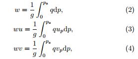
Bulk models take the entirety of the water column. F or an integral water column, the atmosphericwater balance equation is given as follows:
wherewhere w is the precipitable water contained in the unitarea column of air; E is the ev aporation; P is the precipitation; q is the specific humidity; u and v st and for zonal and meridional wind velocities, and up and vpst and for wind velocities at different pressure levels; g is the gravitational acceleration; and ps is thesurface pressure.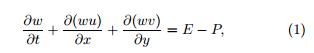
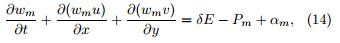
When tagging water from a specific region, according to the well-mixed assumption, there is
where the subscript m refers to the tagged water fromthe source region. The balance equation of the atmospheric moisture from the source region is expressedas follows:When in the source region, δ = 1; otherwise, δ = 0. 3. 2 Equations for b ackward moisture tracking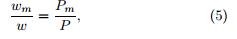
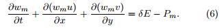
Section 3. 1 provides a mathematical solution ofwater from ev aporation to precipitation. In the sourcereceptor process, the tagged water conserves to Eq. (6). Source A's contribution to receptor B's precipitation in a period can be measured. If we inverse thetime axis, when precipitation returns into the atmosphere as water vapor and ev aporation sinks to theground as ground water, the precipitated water willreturn to its original source(s). A similar process applies in the forward method. If we change precipitation into source and ev aporation into sink term, thenew atmospheric water balance equation is as follows:
where u and v will also change sign. The well-mixedassumption still holds. Therefore, there is
where the subscript m refers to the tagged water fromthe precipitation region. When precipitation reversesback to ev aporative source(s), part of it sinks to theground in proportion to its moisture fraction, whichis E × wm=w. According to the basic conserv ationequation, i. e., Eq. (7), the atmospheric water balanceequation of precipitation reversing is given as follows:where δ = 1 for the tagged source region(precipitationas source), and δ = 0 otherwise. 3. 3 Numerical implementation
The model used here is a modification of WAM. The numerical implementation is similar. The numerical scheme for the moisture balance equations is anexplicit one, and the advection is done with centraldifference scheme at the grid boundaries. The difference scheme is not a general forward-time centralspace(FTCS)method, since the precipitable waterserves as a known variable, and we always substitutethe calculated value at the next time step. The grid is1. 5°× 1. 5° and approximated by trapezoids. The horizontal moisture fluxes, wu and wv, are transformedinto unit cubic meter of liquid water per time stepover grid boundaries; vertical fluxes, E and P, aretransformed into unit cubic meter per time step overa grid cell; and precipitable water, w, is transformedinto unit cubic meter over a grid cell. T o calculatethe column moisture and horizontal moisture flux, thespecific humidity and wind speed at ground level areinterpolated or extrapolated linearly .
To be in harmony with the explicit scheme, thescheme needs to fulfill the Courant-F riedrichs-Lewycondition to keep the computation stable. In this case, the condition is: |wu| + |wv| < w. The time step is setto 0. 5 h in van der Ent et al. (2010). When the sametime step is set in this study, the result still diverges. Diverged grids always occur in polar regions, where wis much smaller than in midlatitude grids. Therefore, in the present study, we made a modification by combining 10 rows of grids on each polar edge into one rowof grids. In WAM, the north and south edges are generally left alone, since including them has barely anyeffect. When the north and south boundary grids arecombined, these new boundaries cannot be left alone. They are put in the recycling computation in the modified WAM.
Region A's contribution to region B's precipitation in the forward tracking method is calculated asfollows:
where P(t; x; y|B)is the precipitation over regionB, wm(t; x; y|B)is the air moisture of origin A, wm(t; x; y|B)is the total air moisture, and t spans theprecipitation period.
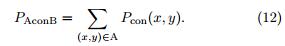
In the backward tracking method, the spatial contribution map for region B's precipitation is easily obtained. F or each grid, its contribution quantity is
where t spans the whole pre-precipitation ev aporationtime, which may begin more than 10 days before precipitation. F or region A, it is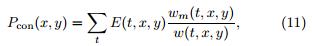
The residence time for atmospheric moisturevaries with time and space(Trenberth, 1998). If wesuppose that the residence time for A is k days at a certain time, any moisture from A will have no influenceor will be so small that is has a negligible influenceon precipitation k days later. Then, if t in Eqs. (10) and (11)approaches infinity, the results of PA2B and PAconBshould approach each other. In practice, themoisture always decays in an e-folding mode, and t isfinite, so the two results may be approximate but notidentical. Even when there are errors in the data, thebasic moisture balance equation does not close, and the methods of dealing with residual will also influencethe results. The residual ff is added to the moisturebalance equation as in Dominguez et al. (2006):
and Eq. (6)changes into and Eq. (9)changes similarily . There are several waysto deal with the residual, such as considering it as apart of precipitation(Goessling and Reick, 2011)orassuming that αm/α = wm/w as in Yoshimura et al. (2004)or van der Ent et al. (2010). In this paper, thelatter approach was adopted.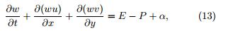
Forward and backward difference schemes basedon the simplest one-v ariable cases usually do notmatch. To reduce the imbalance associated with different difference schemes applied to unclosed data, aset of experiments were performed, where we addedthe residual term α in the forward tracking model butnot in the backward tracking model(αm= 0 in thelatter model). This is another modification we madeon the WAM. Accordingly, another set of backwardtracking with the residual was done for comparison.
Numaguti(1999)found that the average time ofwater vapor residing in the atmosphere was 10 days. Other studies such as Trenberth(1998) and van derEnt and Savenije(2011)investigated extensively theresidence time of water vapor in the atmosphere. Theyrevealed that the residence time changes with bothgeographic location and season. In this paper, we assume that the residence time is around 20 days. In thepresent case, the precipitation period was from 18 to20 July 2007. Based on the 20-day residence time assumption, the moisture before 1 July had a negligibleinfluence on the precipitation. The ev aporative sourcewas traced back to 1 July . F urthermore, in forwardtracking, the beginning date was set on 1 July and the ending date on 20 July . Then, the precipitationcontribution from different sources during the extremeprecipitation event was calculated. The source regionswere determined according to the backward trackingdescribed in Section 4. We also used the GPCP datain comparison with the ERA-I data. 4. Results
According to the ERA-I precipitation data, theaccumulated precipitation in Sh and ong during thethree days of the extreme event was 1. 45 × 1010m3(58. 7 mm in depth). According to GPCP data, itwas 1. 56 × 1010m3(63. 2 mm). Through the backward moisture tracking model, the contributed moisture from each grid in every time step was recorded. The accumulated contribution to Sh and ong's precipitation from each grid from 1 to 20 July, based on backward tracking without the residual, is shown in Fig. 2. The source grids contribute 1. 42 × 1010m3of waterin total, which accounts for 98% of the precipitation, with around 0. 03 × 1010m3left hanging in the air "tobe precipitated. " Backward tracking with GPCP precipitation was also performed. The moisture contribution pattern of GPCP is only slightly different thanthat of the ERA-I, with the exception that the rangeof the same contribution level exp and ed. In backwardtracking considering the residual, the grids contribute1. 14 × 1010m3of water in total, with 0. 02 × 1010m3of water left in the air. When the residual was added, the tagged water from Sh and ong precipitation did notconserve. In terms of water balance, backward tracking without the residual provides a better result.
 |
| Fig. 2. The contributions(shaded; mm)of grids as sources to the Sh and ong precipitation. ERA-I data are applied, and the residual is not considered. The squares denote the regions chosen for forward moisture tracking. The vectorsindicate horizontal moisture flux averaged from 1 to 20 July . |
The spatial contributions based on ERA-I withresidual are shown in Fig. 3. The spatial patterndiffers a little from the backtracking without residual. According to the tracking results, some watersources even traversed the Arabian Sea to reach theeast coast of Africa and cross the equator. But thefurther they are from the sink, the smaller the contribution of these grids to Sh and ong precipitation, sincemuch of the moisture is depleted on the way . Thehigher contribution values appear upwind near theprecipitation region, where the local ev aporation and the tagged moisture ratio are high. The contributionsare more concentrated on l and , especially from northern to southwestern China.
 |
| Fig. 3. As in Fig. 2, but with the residual. |
Since the results of the forward tracking methodmust be somewhat consistent with those of the backward tracking method, three sample squares werepicked as water sources to perform forward tracking. These regions were picked according to the grid contribution gradient. They belong to three different contribution levels, as shown in Fig. 2. Each comprises4 × 4 grid cells. According to the results of backwardtracking shown in Fig. 2, the three regions contribute(from near to far)about 1. 92 × 109, 1. 06 × 109, and 3. 53 × 108m3of water respectively, accounting for13. 3%, 7. 3%, and 2. 4%, respectively .
For GPCP data with the same residual scheme, the resulting contributions are 1. 93 × 109, 1. 12 × 109, and 3. 74 × 108m3(12. 3%, 7. 2%, and 2. 4%), respectively . For the ERA-I data considering the residual, the results are 1. 71 × 109, 8. 67 × 108, and 1. 75 ×108m3. As mentioned in previous sections, in order to reduce the imbalance effect of different difference schemes on imbalanced data, the forward tracking method considering the residual was implementedfor comparison with the backward tracking methodwithout the residual. Applying the forward trackingmodel, the three source regions' contributions are 1. 92× 109, 1. 06 × 109, and 3. 53 × 108m3, which are thesame as the results calculated by the backward tracking method. The GPCP forward tracking experimentproduce results of 1. 93 × 109, 1. 12 × 109, and 3. 74 ×108m3. The two results agree decently .
Region 2's contribution based on ERA-I precipitation data from 18 to 20 July is used as an examplein Fig. 4. The ev aporated water leaves the sourceregion and precipitates wherever it flows. As seen inFig. 4, most of region 2's ev aporation does not fallinto its source. When there is heavy rain in the downwind direction and the tagged moisture ratio is high, the recycled precipitation from region 2 is also high. The major sink is in the middle of China, downwindof the source region, where precipitation is the highest(ERA-I dataset; Fig. 1) and gradually reduces asmoisture flows away.
 |
| Fig. 4. Recycled precipitation(mm)from region 2(denoted by the white box). |
It does not seem to be coincidental that the resultsof forward and backward tracking match completely inthe Sh and ong rainfall case. Several other experimentsconducted by us also support the idea that forwardtracking with the residual agrees with backward tracking without the residual. There seems to be a mathematical necessity in the difference scheme. Accordingto experiments conducted on this issue, we could express this relationship accurately as follows: SourceA's ev aporation at time t1 has an influence(contribution)f1(through forward tracking method with residual)on receptor B's precipitation at time t2. Then, through backtracking without the residual, the precipitation of B at time t2reverses its way back to sourceA. The contribution of source A at time t1denoted asf2 equates with f1.
The analysis of such situations is complex. Whenmoisture from source A spreads to sink B, there aremany paths of A reaching B. We attempt to simplifythis complexity and consider just one of the paths. Other cases are additions to or derivations of this situation. Meanwhile, the flows of the grids along thepath are various. To further simplify, consider thatthere are only flows along this path, and the flows arein a single direction from A to B. Then, the questionbecomes how the ev aporation E of A at time t1 influences the precipitation P of B at time t2in this flowpath. However, it is still hard to make direct comparisons between forward tracking and backward trackingresults, since the iterations are very complex. Withinseveral time steps, the iterations will make the expressions extraordinarily large, and it will be di°cult tocompare the expressions directly . We try to sort outthe analysis through the following steps.
Step 1: The grid next to A is denoted as N1. Prove that the statement holds between grid A and its neighboring grid N1, which is much easier to obtain. Then the statement holds between grid N1 and the next grid N2.
Step 2: Prove that the statement holds betweengrid A and grid N2. A's ev aporation transfers a volume to grid N1, denoted as E1, and N1 and N2 conform to the statement. E1can be viewed as ev aporation from N1. In the next time step, the left ev aporation of E in A transfers another volume to N1, whichis also viewed as ev aporation of N1. Then, the statement between A and N2can be precisely deduced, sois N1to N3, N2to N4, . . ., and so on.
Step 3: If the statement between N1 and grid Nist and s, it is inferred that it st and s between A and Nithrough Step 2 with N1being a pivot point. Then, along the path from A to B, the statement st and s between A and B. This completes the demonstration ofthe steps. In the demonstration, there is a strongercondition than stability to meet when the two results completely agree; that is, |wu| + |wv| + E
The accuracy of the results needs further discussion. First, there is a basic assumption in both models:the assumption of well-mixed atmosphere. In practice, the well-mixed assumption may not be satisfied. Fitzmaurice(2007)pointed out three categories of precipitation that correspond to different mix conditions. One is convection, where the precipitation has a local bias since local moisture contributes more than itsproportion. The second is upper troposphere storms, where the advected moisture contributes more. Thelast is frequent deep convection, where the originalwell-mixed assumption is valid, such as the rainfallsin Thail and in the monsoonal period( Yoshimura et al., 2004). Several methods have been proposed to account for the non-well-mixed condition(e. g., Burde, 2006; Fitzmaurice, 2007), but they depend on empirical parameters that are seldom available and are notavailable on transient timescales. Van der Ent et al. (2013)divided their original WAM into a two-layermodel to account for this condition. Within each layer, it is well-mixed. The results match well with a regionalclimate model-based moisture tracking method, whichis taken for reference.
Second, the unclosed nature of reanalysis data introduces uncertainties. In this study, the GPCP product serves as another precipitation dataset that provides more reliable spatial distribution of rainfall. Theresulting contribution map derived from GPCP datais only slightly different than that from the ERA-Idata, with the exception that the GPCP map is alittle higher and the range of the same contributionlevel exp and s more. Besides precipitation, ev aporation is a less reliable variable. As analyzed before, thesource region's ev aporation and the sink region's precipitation are crucial volumes that directly influencethe results.
Third, different schemes for dealing with theresidual also influence the final result. The backwardtracking with residual brings more spatial variationsthan changing a precipitation dataset in this study, because changing the precipitation only influences themagnitude of the result; the spatial pattern basicallystays the same. The residual is more spatially variable, which brings more spatial variations to the result.
Due to many uncertainties, the results we obtained from either forward tracking or backward tracking are more suitable for reference than for accuracy . The spatial pattern of recycling moisture is more reliable than the numerical value.
In this paper, the moisture sources for the selected rainfall event are concentrated to the southwestof Sh and ong as in Figs. 2 and 3, which are of terrestrial origin. The study of Chen et al. (2011), whoinvestigated moisture sources in a similar case usinga Lagrangian method, found that the terrestrial ev aporation is more important than oceanic source. Ofthe terrestrial ev aporation, they found that the IndoChina Peninsula, Sichuan, and Y unnan provinces inChina contributed more. Their result is consistentwith the result in this paper.
For summer precipitation in an extratropical arealike Sh and ong Province of China, the precipitationmight be of convection type. In this case, the precipitation has a local bias. As in Fig. 2, the nearer tothe precipitation sink upwind, the higher the proportion that the ev aporation there becomes involved inthe precipitation process; the further away, the lowerthe proportion. Thus, there is an aggregated effect inthe upwind area near the precipitation sink, where thearea's moisture contribution counts more than calculated and dispersed effect in regions that are furtheraway . Similarly, there is a more dispersed effect whenthe tagged water precipitates downwind far away fromthe source region(as in Fig. 4). 6. Conclusions
This paper applies a modification WAM to trackthe sources of an extreme precipitation event in Sh and ong Province of China from 18 to 20 July 2007. Inthe experiments of forward tracking and backwardtracking, we found that backward tracking withoutthe residual agreed with forward tracking with consideration of the residual. This result is validated byexperiments conducted in this case study and othercases not shown here. We found that there is a mathematical necessity in the difference schemes, so weprovided key demonstration steps and the conditionsunder which the two results completely matched. Inaddition, we also found that forward tracking withoutthe residual agreed with backward tracking with theresidual under the same conditions.
Backward moisture tracking(without residual)ofthe Sh and ong precipitation event in July 2007(nearly58. 7 mm in 3 days, based on the ERA-I data)indicated that the three source regions contribute(fromnear to far)7. 8, 4. 3, and 1. 4 mm of water, which account for 13. 3%, 7. 3%, and 2. 4%, respectively . Usingthe GPCP data(63. 2 mm in total), the source regionscontribute 7. 8, 4. 5, and 1. 5 mm, which account for12. 3%, 7. 2%, and 2. 4%, respectively . The forwardtracking method with residual precisely matches theseresults. In backward moisture tracking(with residual)based on ERA-I data, the results are 6. 9, 3. 5, and 0. 7mm, which are not the same as backward moisturetracking(without the residual). The results of forward tracking(without the residual)precisely matchthe results of backward tracking(with the residual).
Due to uncertainties in data, different schemes fordealing with the residual, and the well-mixed assumption, the moisture tracking result is more suitable forreference. However, the spatial pattern is more reliable. In any case, we are able to determine that themoisture in this Sh and ong precipitation event originated mostly from the near upwind area of SouthwestChina, which is of terrestrial origin, and the neighboring West Pacific contributed little.
| [1] | Bosilovich, M. G., and S. D. Schubert, 2002: Water vapor tracers as diagnostics of the regional hydrologic cycle. J. Hydrometeorol., 3, 149-165. |
| [2] | —-, and J. D. Chern, 2006: Simulation of water sources and precipitation recycling for the MacKenzie, Mississippi, and Amazon river basins. J. Hydrometeorol., 7, 312-329. |
| [3] | Brubaker, K. L., D. Entekhabi, and P. S. Eagleson, 1993: Estimation of continental precipitation recycling. J. Climate, 6, 1077-1089. |
| [4] | Budyko, M. I., and O. A. Drozdov, 1953: Zakonomernosti vlagooborota v atmosfere (Regularities of the hydrologic cycle in the atmosphere). Izv. Akad. Nauk SSSR, Ser. Geogr., 4, 5-14. |
| [5] | Burde, G. I., 2006: Bulk recycling models with incomplete vertical mixing. Part I: Conceptual framework and models. J. Climate, 19, 1461-1472. |
| [6] | —-, and A. Zangvil, 2001: The estimation of regional precipitation recycling. Part II: A new recycling model. J. Climate, 14, 2509-2527, doi: 10.1175/1520-0442(2001)014 <2509:TEORPR>2.0.CO;2. |
| [7] | Chen Bin, Xu Xiangde, and Shi Xiaohui, 2011: Estimating the water vapor transport pathways and associated sources of water vapor for the extreme rainfall event over east of China in July 2007 using the Lagrangian method. Acta Meteor. Sinica, 69, 810-818. (in Chinese) |
| [8] | Dirmeyer, P. A., and K. L. Brubaker, 1999: Contrasting evaporative moisture sources during the drought of 1988 and the flood of 1993. J. Geophys. Res., 104, 19383-19397. |
| [9] | —-, and —-, 2007: Characterization of the global hydrologic cycle from a back-trajectory analysis of atmospheric water vapor. J. Hydrometeorol., 8, 20-37. |
| [10] | Dominguez, F., P. Kumar, X. Z. Liang, et al., 2006: Impact of atmospheric moisture storage on precipitation recycling. J. Climate, 19, 1513-1530, doi: 10.1175/JCLI3691.1. |
| [11] | Draxler, R. R., and G. D. Hess, 1998: An overview of the HYSPLIT? 4 modeling system for trajectories, dispersion, and deposition. Aust. Meteor. Mag., 47, 295-308. |
| [12] | Drozdov, O. A., and A. S. Grigor’eva, 1965: The Hydrologic Cycle in the Atmosphere. Israel Program for Scientific Translations, 282 pp. |
| [13] | Eltahir, E. A. B., and R. L. Bras, 1994: Precipi-tation recycling in the Amazon Basin. Quart. J. Roy. Meteor. Soc., 120(518), 861-880, doi: 10.1002/qj.49712051806. |
| [14] | Fitzmaurice, J. A., 2007: A critical analysis of bulk precipitation recycling models. Ph.D. thesis, Mass. Inst. of Technol., Cambridge. |
| [15] | Fu Xiang, Xu Xiangde, and Kang Hongwen, 2006: Re-search on precipitation recycling during Meiyu season over middle-lower reaches of Changjiang River in 1998. Meteor. Sci. Technol., 34, 394-399. (in Chinese) |
| [16] | Gimeno, L., A. Stohl, R. M. Trigo, et al., 2012: Oceanic and terrestrial sources of continental precipitation. Rev. Geophys., 50, doi: 10.1029/2012RG000389. |
| [17] | Goessling, H. F., and C. H. Reick, 2011: What do mois-ture recycling estimates tell us? Exploring the extreme case of non-evaporating continents. Hydrol. Earth Syst. Sci., 15, 3217-3235, doi: 10.5194/hess-15-3217-2011. |
| [18] | —-, and —-, 2013: On the “well-mixed” assumption and numerical 2-D tracing of atmospheric moisture. Atmos. Chem. Phys., 13, 5567-5585, doi: 10.5194/acp-13-5567-2013. |
| [19] | Kurita, N., A. Numaguti, A. Sugimoto, et al., 2003: Relationship between the variation of isotopic ratios and the source of summer precipitation in eastern Siberia. J. Geophys. Res. Atmos. (1984-2012), 108(D11), doi: 10.1029/2001JD001359. |
| [20] | —-, N. Yoshida, G. Inoue, et al., 2004: Modern isotope climatology of Russia: A first assessment. J. Geophys. Res. Atmos. (1984-2012), 109(D3), doi: 10.1029/2003 JD003404. |
| [21] | Numaguti, A., 1999: Origin and recycling processes of precipitating water over the Eurasian continent: Experiments using an atmospheric general circulation model. J. Geophys. Res., 104, 1957-1972, doi: 10.1029/1998JD200026. |
| [22] | Ralph, F. M., P. J. Neiman, G. A. Wick, et al., 2006: Flooding on California’s Russian River: Role of atmospheric rivers. Geophys. Res. Lett., 33, doi: 10.1029/2006GL026689. |
| [23] | Stohl, A., C. Forster, A. Frank, et al., 2005: Technical note: The Lagrangian particle dispersion model FLEXPART version 6. 2. Atmos. Chem. Phys., 5, 2461-2474. |
| [24] | Trenberth, K. E., 1998: Atmospheric moisture residence times and cycling: Implications for rainfall rates and climate change. Climate Change, 39, 667-694. |
| [25] | Van der Ent, R. J., H. H. G. Savenije, B. Schaefli, et al., 2010: Origin and fate of atmospheric moisture over continents. Water Resour. Res., 46, doi: 10.1029/2010WR009127. |
| [26] | —-, and —-, 2011: Length and time scales of atmospheric moisture recycling. Atmos. Chem. Phys., 11, 1853-1863. |
| [27] | —-, and —-, 2013: Oceanic sources of continental precipitation and the correlation with sea surface temperature. Water Resour. Res., 49, 3993-4004. |
| [28] | —-, O. Tuinenburg, H.-R. Knoche, et al., 2013: Should we use a simple or complex model for moisture recycling and atmospheric moisture tracking? Hydrol. Earth Syst. Sci. Discuss., 10, 6723-6764. |
| [29] | Yoshimura, K., T. Oki, N. Ohte, et al., 2003: A quantitative analysis of short-term 18O variability with a Rayleigh-type isotope circulation model. J. Geophys. Res., 108(D20), doi: 10.1029/2003JD003477. |
| [30] | —-, —-, —-, et al., 2004: Colored moisture analysis estimates of variations in 1998 Asian monsoon water sources. J. Meteor. Soc. Japan, 82, 1315-1329, doi: 10.2151/jmsj.2004.1315. |
| [31] | —-, M. Kanamitsu, D. Noone, et al., 2008: Historical isotope simulation using reanalysis atmospheric data. J. Geophys. Res. Atmos. (1984-2012), 113, D19108, doi: 10.1029/2008JD010074. |