 2013, Vol. 28
The Chinese Meteorological Society
Article Information
- WANG Jinxin, PAN Yinong, WANG Shicheng. 2013.
- A Numerical Study of the Evolution of a Mesoscale Convective Vortex on the Meiyu Front
- J. Meteor. Res., 28(6): 889-909
- http://dx.doi.org/10.1007/s13351-013-0509-9
Article History
- Received January 29, 2013;
- in final form June 16, 2013


2 Lianyungang Meteorological Bureau, Lianyungang 222006
The continued development of progressively more advanced observational instrumentation with improved precision has led to the detection of various mesoscale meteorological phenomena, including mesoscale convective vortices(MCVs). MCVs were first observed in the stratiform region of tropical mesoscale convective systems(MCSs)(e.g., Houze, 1977; Gamache and Houze, 1982). These vortices have since been shown to be more prominent in midlatitude MCSs(Zhang and Ni, 2010). Investigations of MCVs in the 1980s and early 1990s were limited to studies using routine observational data, such as satellite retrievals, radar, and soundings. These early studies were only able to reveal some of the basic features of MCVs. For example, Menard and Fritsch(1989)showed that a mid-level mesoscale vortex can develop within a mature or decaying mesoscale convective complex(MCC). Fritsch et al.(1994) investigated a longlived warm-core vortex that intensified after every cycle of convection within the vortex circulation. They concluded that a vortex could generate new convection provided favorable environmental winds and suffcient low-level values of equivalent potential temperature(θe). They also found that this secondary convection could in turn amplify the vortex. The lack of highresolution observations has forced researchers to turn to numerical models for more detailed examinations of MCVs. Raymond and Jiang(1990)famously proposed a mechanism for how MCSs could become long-lived and self-sustaining. Zhang(1992) and Chen and Frank(1993)captured several types of MCVs. Zhang(1992)identified a cooling-induced mesoscale vortex in the trailing stratiform region of a midlatitude squall line. This vortex resulted primarily from the tilt of the downdraft and the convergence of the interface between front-to-rear flow and rear-to-front flow. Chen and Frank(1993)concluded that the formation of mesoscale vortices in the stratiform regions of MCSs results primarily from reduction of the Rossby deformation radius.
Many recent studies have used a "top-down" conceptual model of MCV development to elucidate potential links between MCVs and the process by whichtropical cyclones(TCs)extend downward to the seasurface(thereby inducing air-sea interactions that leadto rapid intensification). Rogers and Fritsch(2001)showed that amplification of a mid-level warm corecould lower surface pressure, inducing(through gradient wind balance)a transition from an anticycloniccirculation above the cold pool to a cyclonic circulation. Davis and Galarneau(2009)showed that MCVscan also penetrate downward to the surface via vertical coupling between a mid-level MCV and a low-levelline-end vortex formed by the effects of eddy fluxes onthe outflow boundary. The downward penetration ofan MCV over l and could lead to surface frontogenesis and organized precipitation(Galarneau et al., 2009).
To date, few studies have examined MCVs overeastern China during the Meiyu season. In this paper, we present a simulation of a Meiyu season MCV thatformed in eastern China in 2008, lasted for more thantwo days, and penetrated to the surface. Two organized convective systems formed within the MCV circulation during its lifetime. The first convective cyclewas associated with the rapid formation of the MCV, while the second was associated with the intensification of the MCV and its downward extension to thesurface. We explore the processes that contribute to and control the genesis, intensification, and downwardpenetration of this MCV.
The primary tool used in the simulation study isthe Advanced Research WRF(Weather Research and Forecasting)model(ARW). Section 2 contains a description of the model setup and the simulation design.Section 3 provides a validation of the model resultsagainst observations. Section 4 presents an analysis ofthe simulated vorticity, temperature, and energy budgets, as well as the Rossby radius of deformation. Theresults are discussed in Section 5.2. Model description and data
ARW is a non-hydrostatic model with a terrainfollowing vertical coordinate(σ). This simulation isperformed using ARW version 3.3.1. The model domain for this simulation consists of three meshes: anouter mesh with a horizontal resolution of 9 km and two two-way interactive inner meshes, each with a horizontal resolution of 3 km(Fig. 1). The outer domain(D01)contains the MCV, the parent MCS, and thesecondary MCS from genesis to dissipation. The firstinner domain(D02)covers the area in which the MCVwas generated by the parent MCS. The second innerdomain(D03)is centered on the secondary MCS thatdeveloped within the MCV. Table 1 lists the key aspects of the model formulation. We use the Thompsonmicrophysics scheme, which has been shown to produce a more extensive stratiform region than the Linet al.(1983)scheme(Davis and Galarneau, 2009; Liu et al., 2011).
 |
| Fig. 1. Terrain height(m)within the outer domain D01 and the two inner meshes D02 and D03. |

The outer domain of the ARW is initialized using 6-h output from the global analysis data of atmosphere(GANAL), which was the operational forecast model for the region run by the Japan Meteorological Agency at the time of the MCV. The data cover the area 10°-60°N, 110°-160°E with a resolution of 0.25° in longitude and 0.2° in latitude. Kinematic and thermal data are provided on 21 vertical pressure levels, while moisture is provided on 12 vertical levels. The portion of D01 that is not covered by GANAL data is initialized using 6-h NCEP GFS FNL data with a 1.0°×1.0° horizontal and a 50-hPa vertical resolution(25 hPa in lowest 100 hPa). The two inner domains D02 and D03 are initialized from the outer domain. The analysis presented in this paper focuses exclusively on the output from D01.
We take observations of rainfall from the realtime hourly precipitation rates produced by theTropical Rainfall Measuring Mission(TRMM)with a 0.1°×0.1° horizontal resolution(http://www.eorc.jaxa.jp/TRMM/index−e.htm). This dataset coversthe tropics and extratropics between 60°S and 60°N.We also use hourly observations of infrared brightness temperatures from the Multi-functional Transport Satellite 1R(MTSAT-1R)(http://www.jma.go.jp/jma/jma-eng/satellite), which have been interpolated onto a 0.05°×0.05° grid within 20°S–70°N, 70°–160°E.3. Case description and model verification
We briefly describe the MCV event and validate the model results against observations. Figure 2 shows a series of infrared images taken by the MTSAT-1R satellite at 6-h intervals, while Fig. 3 shows observations of cumulative precipitation over the same 6-h intervals. The region where the MCV formed was covered by a large area of stratiform cloud, with strong horizontal wind shear and a mesoscale trough oriented west-east(Figs. 2a and 2b). Accordingly, the intense rainfall region of the MCS contained an area of high vorticity even before the genesis of the MCV(Figs.3a and 3b). A mesoscale cyclone formed in the stratiform region 6 h later, resulting in a typical vortical cloud(Fig. 2c). The formation of additional convection near the center of the MCV(Figs. 2d and 2e)was accompanied by the formation of a new center of positive vorticity(Figs. 3d and 3e). This vorticity center was slightly displaced relative to the location of the previous vorticity center, resulting in an elongated vortex(Figs. 2f–h and 3f–h)(Rogers and Fritsch 2001). Two mesoscale convective complexes(MCCs)were located to the south of the MCV by 1200 UTC 26 July(Fig. 2h). Although one might expect the MCV to be affected by these two MCCs, examination of the GANAL data indicates that it was not. This may be due to deficiencies in the GANAL data. Our use of these data as initial conditions for the simulation may in turn cause discrepancies between the model output and observed conditions. The model simulation does not produce any MCCs to the south of the MCV at 1200 UTC 26 July(see Fig. 4g).
 |
| Fig. 2. Cloud-top temperature(℃)observed by the MTSAT-1R satellite(shadings) and 500-hPa winds(streamlines)from GANAL for the period 1800 UTC 24 to 1800 UTC 26 July 2008. The letter V denotes the center of the MCV. |
 |
| Fig. 3. Cumulative precipitation(mm; shadings)from TRMM 6 h prior to the indicated time, along with instantaneous winds, relative vorticity(black contours), and temperature(grey contours)at 500 hPa from the GANALdata. |
 |
| Fig. 4. Simulated 500-hPa winds and maximum reflectivity(dBZ). The letter V denotes the central location of the MCV, S1 the parent MCS, and S2 the secondary MCS. |
Figure 4 shows the structure of the simulatedMCV at 500 hPa. The ARW simulates the shape, size, and location of the MCV well. A small-scale vortex initially formed to the north of the parent MCS(Fig. 4a), and then gradually evolved into a stratiformembedded mesoscale cyclonic vortex(i.e., the MCV)(Fig. 4b). The MCV persisted even after the dissipation of the parent MCS(Fig. 4c). The developmentof secondary organized convection on the down-shearside of the MCV(Fig. 4c)was followed by the formation of a second cyclonic vortex center to the northof the fully-developed secondary MCS(Fig. 4d). Astrengthened and elongated mesoscale vortex formedwhen the original MCV merged with this new vortex(Fig. 4e). Organized convection was replaced by scattered convective cells during the latter portion of theMCV event(Figs. 4f–h).
Figure 5 shows the vertical structure of the simulated vortex. The genesis location of the vortex wasprimarily determined by the location of a broad regionof southerly wind, with a maximum wind speed of 16m s−1 in the mid troposphere(Fig. 5a). This regionof southerly wind and a narrow column of northerlywind(located to the west of the vortex center with amaximum at upper levels; see Fig. 5a)comprised theinitial cyclonic circulation of the vortex. The vortexwas therefore asymmetrical during its genesis stage.The initial horizontal distance between the two windmaxima was no more than 50 km. The MCV amplified, became increasingly symmetrical, and penetrateddown to lower levels as the area of northerly wind exp and ed(Figs. 5b and 5c). The development of thesecondary MCS destroyed the symmetry of the vortex, accelerating the southerly winds and decelerating thenortherly winds at low and mid levels(Figs. 5d and 5e). These changes were caused by the developmentof a deep layer of strong southerly wind that suppliedmoist, warm air to the convection in the new MCS.The areas of southerly and northerly winds again approached balance after the dissipation of the convection; accordingly, the MCV grew more symmetrical(Figs. 5f and 5g)with a distance of more than 250km between the wind maxima. The lack of diabaticheating and constant frictional dissipation by the environment gradually weakened the mid-level MCV. Bycontrast, the low-level cyclonic circulation intensifiedduring this period, with southerly wind maxima evenexceeding that of the mid-level MCV. The followingsections discuss the reasons for the genesis, intensification, and penetration of the MCV.
 |
| Fig. 5. Simulated meridional wind(m s−1; contours) and vertical velocity(m s−1; shadings)along an east-west crosssection through the center of the MCV at 6-h intervals from(a)0000 UTC 25 to(i)0000 UTC 27 July. The contourinterval is 2 m s−1. Dashed lines indicate northerly wind. |
Previous work on MCV dynamics has been basedprimarily on theories of vorticity, temperature, and energy budgets, and the Rossby radius of deformation.These theories are interdependent when applied tovortex dynamics. The vorticity budget concerns thekinematic aspects of the vortex, while the temperature budget concerns the thermal aspects. The energybudget reveals links between kinematics and thermodynamics and the conversion of energy from one typeto another. The local Rossby radius of deformationconcerns the interconnection between the MCS and the MCV, and reveals positive feedbacks between theMCS and the MCV.
Most previous studies have focused on only one or two of these four aspects. None has fully investigated the dynamics of the vortex throughout its lifetime examining all the four aspects. In this section, we present a series of budget analyses based on theresults of our simulation to fill this gap.4.1 Vorticity budget and kinematic evolution
The vorticity budget is the most commonly analyzed budget in research on MCV dynamics(e.g., Zhang and Fritsch, 1987; Bartels and Maddox, 1991;Zhang, 1992; Chen and Frank, 1993; Yu et al., 1999;Rogers and Fritsch, 2001; Kirk, 2003; Knievel and Johnson, 2003; Davis and Galarneau, 2009). Previous studies have shown that stretching effects aredominant for most MCVs(e.g., Zhang and Fritsch, 1987; Bartels and Maddox, 1991; Rogers and Fritsch, 2001; Kirk, 2003; Knievel and Johnson, 2003; Davis and Galarneau, 2009); however, other vorticity budgetterms may dominate under certain special cases(e.g., Zhang, 1992; Yu et al., 1999; Davis and Galarneau, 2009). Stretching-dominated MCVs usually form and evolve in stratiform regions, while tilting-dominated MCVs are often located in convective regions(e.g., Davis and Galarneau, 2009).
We investigate the vorticity dynamics of the MCVby analyzing a renewed form of the vorticity equation(Haynes and McIntyre, 1987; Davis and Galarneau, 2009). The st and ard form of the vorticity equation iswritten as
where ζ is relative vorticity, η the absolute vorticity, ωthe vertical velocity in pressure coordinates(x, y, p), vthe horizontal wind vector(with u and v the horizontalvelocity in the x and y directions, respectively),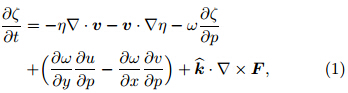
 theunit vector in the vertical direction, and F the horizontal frictional force. Haynes and McIntyre(1987)rewrote Eq.(1)into the divergent formwhere the horizontal vector K is referred to as thevorticity flux vector. Integrating Eq.(2)over a closedhorizontal plane(e.g., the MCV area)yields the renewed vorticity equation in circulation form∂Cwhere C denotes the circulation and
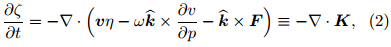
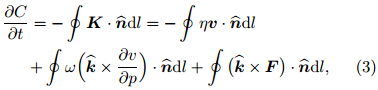
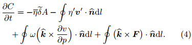
 the outwardunit vector normal to the boundary of the closed horizontal plane. The first term on the right h and sideof Eq.(3)can be decomposed into mean and eddycontributions, yielding the final formOver bars indicate the average taken around theperimeter of the area, primes the perturbation fromthis average value, and tildes the average over the area.The first term on the right h and side of Eq.(4)corresponds to stretching, the second term to the eddyflux, the third term to tilting, and the fourth term tofrictional effects.
The vorticity budget is diagnosed by analyzingthe terms in Eq.(4). The circulation domain is chosen as a square area of 31×31 grid points(270 km×270km). This scale corresponds to the approximate maximum distance between meridional velocity extreme.The results are sensitive to convection and associatedcell-scale variations in vorticity on the edge of the box.For this reason, and to improve the balance of the vorticity budget, we adopt an ensemble approach whereina distribution of budgets is computed at each outputtime. At each output time, the location of the box isperturbed in 9-km increments from its central locationup to a maximum of ±45 km in both the x and y directions. This procedure results in 121 “samples” ofthe vorticity budget(11 × 11). We consider all termsin Eq.(4)but the frictional term. We compare eachterm using the averages of the corresponding distributions. Davis and Galarneau(2009)have described thisanalysis method in detail.
Figure 6 shows vertical profiles of the differentbudget terms averaged over the system-following boxintroduced above. The profile is only shown for levels at 850 hPa and above. Lower levels were below thesurface within the circulation box during the early portions of the analysis period. The budget is generallywell balanced. The stretching and eddy flux contributions are nearly opposite at most levels, as are thevertical variations in these two terms. Positive contributions from stretching at mid levels and eddy fluxat low levels(Fig. 6b)allowed the MCV to attain acoherent vertical vorticity structure between the surface and the mid troposphere(Fig. 6a). Changes inPV were largest at low levels. Moreover, the verticalstructure of changes in PV is nearly the same as thatof vorticity. This result indicates that the low-levelchanges in PV arose mainly from changes in vorticity(particularly those due to eddy fluxes)rather thanfrom diabatic heating.
 |
| Fig. 6.(a)Vertical profiles of box-averaged final vorticity(black), vorticity change over the final 54 h of the simulation(red), sum of rates of change in vorticity due to all terms in the vorticity budget(Eq.(4))except friction(green), and total changes in PV over the final 54 h(blue).(b)Total changes in vorticity due to stretching(black), eddy fluxes(red), and tilting(green). |
Figure 7 shows the temporal evolution of these same three terms in the vorticity budget. During the MCV genesis period(0000–0600 UTC 25 July), the cyclonic circulation strengthened throughout a deep column that extended from low levels upward to the mid troposphere(Fig. 7a). Contributions from stretching and eddy fluxes were both important during this period; however, the layers in which these two terms dominated were different. Stretching dominated vorticity changes at mid levels(550–350 hPa)(Fig. 7b), while eddy fluxes dominated at upper(above 300 hPa) and lower layers(800–550 hPa)(Fig. 7c). The stretching at mid levels resulted from strong mid-level convergence in response to intense upward motion. Vorticity transport into the MCV region from the low-level convective region and the upper-level trough contributed to eddy fluxes at lower and upper levels, respectively.
 |
| Fig. 7. Time-pressure distribution of changes in area-averaged vorticity due to(a)all terms in the vorticity budget(Eq.(4))except friction, (b)stretching, (c)eddy fluxes, and (d)tilting. |
The pattern was similar during the period ofMCV re-intensification(0800 UTC 25–0000 UTC 26July), when new convection emerged near the center of the MCV circulation. The main difference between these two periods was that stretching effectswere also important near the ground during the reintensification period. This difference resulted fromthe strong surface convergence that fed the secondaryconvection. This surface convergence actually appeared before the formation of the secondary MCS, and then grew deeper and stronger as the organizedMCS became fully developed(0800–1800 UTC 25 July)(Figs. 4c and 4d).
Figure 8 shows simulated horizontal winds and absolute vorticity at 850 and 500 hPa at various times during the evolution of the MCV. A mesoscale cyclone formed near the surface at approximately 0800 UTC 25 July(Fig. 8a). The mid-level MCV was suppressed between 0800 and 1200 UTC 25 July, suggesting that the surface cyclone may not have resulted from downward extension of the mid-level MCV and may have been independent of the mid-level MCV. Southerly winds dominated near the surface when the secondary MCS became fully developed, obscuring the near-surface cyclone. The near-surface cyclone then re-emerged when convection ceased at approximately 0600 UTC 26 July(Fig. 8c). The vorticity budget throughout most of the troposphere(800–200 hPa)was dominated by negative contributions from both stretching effects and eddy fluxes, following the dissi-pation of the secondary convection(Figs. 7b and 7c). By contrast, both the stretching and eddy flux contributions remained slightly positive near the surface(900–800 hPa). The strongest circulation of the vortex therefore descended to lower levels(Fig. 5i). The development of this strong surface cyclonic circulation(which was of a similar size with the MCV)below the mid-level MCV produced a deep, vertically erect MCV(Figs. 5i and 8e–f). Although the surface cyclonic circulation resulted in part from eddy flux contribution, it formed almost directly beneath the mid-level MCV. This result contrasts with the findings of Davis and Galarneau(2009), who reported that the surface cyclone initially formed in the outflow boundary before moving beneath the mid-level MCV.
 |
| Fig. 8. Simulated horizontal winds(m s−1; vectors) and absolute vorticity(10−5 s−1; shadings)on the(a, c, e)850- and (b, d, f)500-hPa isobaric surfaces at(a, b)0800 UTC 25, (c, d)0600 UTC 26, and (e, f)0000 UTC 27 July. |
Stretching was the main factor in the rapid intensification of the vortex in the mid tropospherethroughout the lifecycle of the MCV(from 1800 UTC24 to 0000 UTC 27 July). Meanwhile, eddy fluxeswere the main contributor to vortex amplification atlower levels. Negative effects on the mid-level vortex were also mainly due to vorticity export by eddyfluxes. Stretching exerted a dampening effect on theMCV during the dissipation of the MCS. Tilting effects were generally negative and relatively small.4.2 Heat budget and thermal structure
MCVs are often induced by diabatic effects inthe convective regions of MCSs. Analysis of the heatbudget is therefore another important component ofMCV research. Zhang and Fritsch(1987)indicatedthat heating due to processes resolvable at grid scaleswas much greater than heating due to convective scaleprocesses(i.e., parameterized heating). Bartels and Maddox(1991)found that heating maxima were generally located in the upper portion of MCVs, while cooling maxima were generally located in the lowerportion. They also identified cooling near thetropopause and near the surface. The nonlinear balance model introduced by Jiang and Raymond(1995)yielded similar results. Chen and Frank(1993)determined the thermal budget of an MCV by analyzing the thermodynamic equation. They reportedthat the warm anomaly in the upper portion of theMCV was primarily attributable to heating resultingfrom resolvable condensation and evaporation. Thecold anomaly beneath the vortex resulted primarilyfrom vertical motion, including vertical advection and dry-diabatic cooling. Contributions from other terms(such as horizontal advection, diffusion, and parameterized deep convection)were relatively small. Rogers and Fritsch(2001)achieved similar results in a latermodeling study.
We adopt a similar equation used by Chen and Frank(1993), but adapt it to account for radiative heating and the speed of the MCV. We write the thermodynamic equation as
where v is the velocity of the background horizontal wind, c the horizontal velocity of the MCV, ω the vertical velocity, Tv the virtual temperature, qv the water vapor mixing ratio, Cp the the heat capacity of air at constant pressure, Qnc the heating due to large-scale(resolved)microphysics, Qc the heating due to parameterized convection, and Qr the radiative heating. The first term on the right h and side of Eq.(5)represents horizontal advection(TH) and the second term represents vertical advection and adiabatic cooling(TV). The final three terms represent the contributions due to large-scale moist processes(MP), parameterized cumulus convection(CU), and radiation(RA). Strong positive contributions from horizontal advection were mostly confined to the lower and upper troposphere(Fig. 9a). Low-level warm advection acted to maintain the convection, while positive values at upper levels resulted mainly from cold air outflow near the top of the MCS. Vertical advection strongly cooled the atmosphere at most levels(Fig. 9b), especially when convection was active. The distribution of diabatic heating due to large-scale microphysics was approximately opposite to that of vertical advection(Fig. 9c). Parameterized convective heating was positive at all levels, but smaller in magnitude than resolved microphysical heating(Fig. 9d). Radiative heating and cooling was also limited in magnitude, with a distinct diurnal variation between daytime heating and nighttime cooling(Fig. 9e). Overall, these thermal processes heated the upper portion and cooled the lower portion of the atmosphere during the convective period, with a transition to net cooling throughout the atmospheric column after convection ceased(Fig. 9f).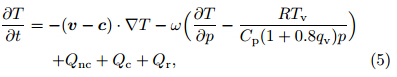
 |
| Fig. 9. Time-pressure distributions of changes in area-averaged temperature(K h−1)due to(a)horizontal advection, (b)vertical advection and adiabatic cooling, (c)diabatic heating from large-scale condensation, (d)diabatic heating from parameterized cumulus convection, (e)diabatic heating from radiation, and (f)all terms on the right h and side ofEq.(5). |
Figure 10 shows the evolution of the thermal structure of the MCV at three vertical levels. The convection acted to heat the atmosphere at upper levels and cool the atmosphere at lower levels. The warm core at upper levels and the cold pool near the surface did not develop at the same pace. The warm anomaly was at a maximum when the MCS was fully developed, while the cold pool was at a maximum as the MCS decayed. These differences resulted from the different thermal characteristics of the MCS at different stages. Fully developed MCSs are typically dominated by processes that heat the atmosphere, resulting in maximal heating and minimal cooling. By contrast, the cooling effect of the MCS is maximal during decay when the MCS is dominated by cold downdrafts. The down shear side of the MCS in the mid troposphere was located under the base of the cloud(where cooling was dominant), while the up shear side was located in a region of dry downdrafts(where warming was dominant). The circulation of the MCV in the mid troposphere(500 hPa)was therefore located in a baroclinic transition zone. This situation ensured that a huge amount of energy was reserved as eddy available potential energy(APE).
 |
| Fig. 10. Simulated winds(m s−1; vectors) and temperatures(℃; shadings)within the MCV at 300(left column), 500(center column), and 750 hPa(right column)at 12-h intervals from(a)–(c)0000 UTC 25 July to(m)–(o)0000 UTC 27 July. |
In Sections 4.1 and 4.2, we have investigated the kinematic and thermal evolution of the MCV. These two aspects have often been considered in isolation. The diabatic effect is often regarded as the fundamental reason for MCV genesis, but few studies have investigated in detail how diabatic processes induce MCVs. Meanwhile, MCVs have long been measured using kinematic metrics, such as those related to circulation and vorticity. Some simulation studies, such as Conzemius et al.(2007) and Conzemius and Montgomery(2010), have investigated the relative contributions of diabatic and baroclinic processes to vortex intensification. Conzemius et al.(2007)investigated MCV formation in a moist neutral environment with weak shear in the context of the Bow Echo and MCV Experiment(BAMEX)campaign. They concluded that the primary contributor to the deepening of an MCV was the eddy APE, which is dominated by diabatic heating. They also noted that baroclinic conversion played a significant role. Conzemius and Montgomery(2010)used numerical simulations to investigate MCV genesis in different environments. They found that the contribution of eddy APE was most important when the background convective available potential energy(CAPE)was also large. The contribution of baroclinic processes increased with larger vertical wind shear. Galarneau et al.(2009)concluded that diabatic heating was the dominant source of eddy APE during the baroclinic transition of a long-lived MCV observed during BAMEX. Jiang and Raymond(1995)provided a detailed analysis of the energy budget of a mature MCS simulated by a nonlinear balance model. They showed a high generation rate of eddy APE, which was persistently transformed into eddy kinetic energy(KE). This KE may in turn amplify the mid-level circulation.
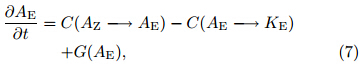
We adopt the method used by Jiang and Raymond(1995)to explore the energy budget of our simulated MCV. The time rates of change of eddy KE and APE can be expressed as
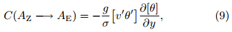
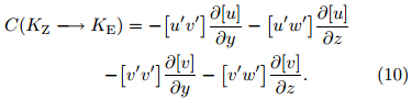
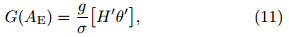
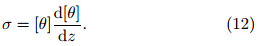
and respectively, where AE and AZ are the eddy and zonalAPE, KE and KZ are the eddy and zonal KE, G(AE)is the generation rate of eddy APE by diabatic processes, and S(KE)results from non-conservative external forces. Terms of the form C(X→ Y)represent conversion rates from energy in form X to energyin form Y . In our analysis, we focus on the threeconversion processes and the generation of eddy APE, neglecting S(KE). The conversion of eddy APE toeddy KE(CAK)is given bythe conversion of zonal APE to eddy APE(CAA)by and the conversion of zonal KE to eddy KE(CKK)byThe generation of eddy APE by diabatic processes(GA)is computed aswhere σ is expressed asThe bracket [ ] denotes a zonal mean, and the primethe departure from the zonal mean. Figure 11 showsa schematic diagram of the links among these types ofenergy.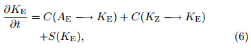

 |
| Fig. 11. Schematic diagram of energy conversion in the MCV region. |
Figure 12 shows density-weighted volume integrals of the rates of energy conversion and generation(Eqs.(8)–(11))as a function of time for this MCV.The generation rate GA and the conversion rate CAKare strongly correlated with the initial and secondaryconvective heating. GA and CAK were both approximately zero when convection ceased. The generationof eddy APE by diabatic heating, which came mostlyfrom convection, was the main source of the energy.We therefore conclude that the convection supportsthe energy of the circulation. By contrast, the conversion CKK occurred primarily when convective activityhad ceased. This period corresponds to the dissipationof the MCV, indicating that the conversion CKK maycontribute to the decay of the MCV. The baroclinicconversion CAA was quite small in this case.
 |
| Fig. 12. Energy conversion rates as a function of time. The black solid line indicates generation of eddy available potential energy(GA), the red dashed line indicates conversion of eddy available potential energy to eddy kinetic energy(CAK), the green dotted line indicates conversion of zonal kinetic energy to eddy kinetic energy(CKK), and the purple short-long dashed line indicates conversion of zonal available potential energy to eddy available potential energy(CAA). |
Table 2 summarizes the terms of the energy budget of a typical 1-m2 column of atmosphere over the54-h lifetime of the MCV(1800 UTC 24 to 0000 UTC27 July). The total conversions of eddy APE and zonalKE to eddy KE were nearly the same, with eddy APEcontributing 46.8% and zonal KE contributing 53.2%.
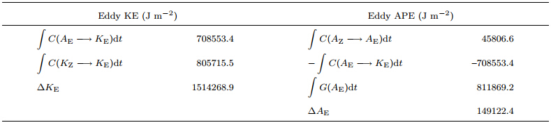
Figure 13 shows the temporal evolution of the mean vertical profile of energy conversion rates in the atmosphere. The upper-level warming due to convection was the main source of energy(Fig. 13e). The eddy APE generated by convective heating was quickly transformed into eddy KE(Fig. 13c). The location of the maximum conversion rate was slightly higher than the center of the MCV. This transformation therefore likely resulted in an upward extension of the MCV. The generation of eddy KE associated with this process is usually accompanied by intense upward motion, which can induce convergence at lower levels(where the mid-level MCV was thus generated by stretching effects). The time period and location of conversion from zonal to eddy KE conformed to the period and location of the MCV’s decay(Fig. 13f). The conversion of zonal KE to eddy KE may have contributed to the decay of the mid-level MCV by transporting straight-line environmental momentum into the MCV region. This transport could destroy the rotational momentum of the MCV even as it enhanced the eddy KE. Positive energy conversion near the surface was small; however, eddy fluxes still caused the formation of a mesoscale cyclone at the surface.
 |
| Fig. 13. Time-pressure distributions of area-averaged(a)eddy KE conversion rate, (b)eddy APE conversion rate, (c)conversion rate of eddy APE to eddy KE, (d)conversion rate of zonal APE to eddy APE, (e)generation rate of eddy APE, and (f)conversion rate of zonal KE to eddy KE. |
One physical hypothesis regarding MCV genesisis that the atmospheric response to a local heat(ormass)source depends on the relative horizontal scalesof the heat source and the local Rossby radius of deformation(Chen and Frank, 1993). The Rossby radiusof deformation is generally defined as
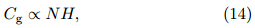
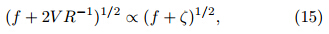
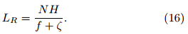
where Cg is the phase speed of an inertia-gravity wave, f the Coriolis parameter, ζ the relative vorticity, and V the tangential component of the wind at the radiusof curvature R(Chen and Frank, 1993; Rogers and Fritsch, 2001). The approximate form of Cg iswhere N is the Brunt-Väisälä frequency and H thescale height of the disturbance. Applying the approximationEq.(13)becomesDurran and Klemp(1982)provided a method for computing the static stability N as a function of relativehumidity: where ε =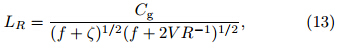
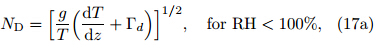
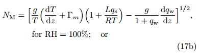
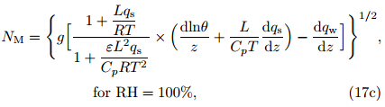
 and qw = qs + qr + qc is the total water content, with qs the saturation mixing ratio, qr therain water mixing ratio, and qc the cloud water mixingratio. Equation(17c)is a very good approximation ofEq.(17b). We compute the static stability using Eqs.(17a) and (17c)(see also Rogers and Fritsch, 2001).
Chen and Frank(1993)hypothesized that the atmospheric response is dominated by the inertial mode if the radius of a local heat source, L, is equal to or greater than LR. This results in a geostrophic adjustment of the wind field to the perturbation in the mass field. Such a mode is called “dynamically large.” On the other h and , the response is dominated by the gravitational mode if L is smaller than LR(i.e., dynamically small). This situation can result in the formation of gravity waves that eliminate the mass anomaly, leaving the rotational wind field largely unaffected. The formation of a vortex in response to diabatic heating is therefore unlikely unless the heating occurs over an area comparable to LR; however, L is generally smaller than LR. We adopt the method applied previously by Chen and Frank(1993) and Rogers and Fritsch(2001)to explore the mechanisms that controlled the formation of the MCV within the MCS.
Figure 14 shows temporal changes in relativehumidity, relative vorticity, static stability, and theRossby radius of deformation within the MCV region. Relative humidity within the MCV region gradually decreased despite the consistent presence of convection around and within the MCV(Fig. 14a). This drying occurred because the moisture was largely confined to low levels. The mid-level moisture was concentrated mainly on the downshear side of the vortex, while the upshear side was warm and dry. Thestatic stability was computed using Eq.(17a). Thestatic stability within the MCV generally increasedwith time(Fig. 14c)due to the increase in  causedby the vertical distribution of heating. Despite thisincrease in static stability, the intensity of the MCVincreased throughout most of the first 36 h, with somedecrease between the two convective periods(Fig. 14b). The temporal variations in vorticity and theRossby radius of deformation were nearly opposite(Fig. 14d), suggesting that the Rossby radius of deformation was primarily controlled by the MCV. Thisresult indicates that the dynamic characteristics of theMCS were primarily determined by the evolution ofthe MCV. Overall, our case differs from that presentedby Rogers and Fritsch(2001). In their case, increasingrelative humidity caused a decrease in static stability and a reduction of the Rossby radius of deformation, enhancing the mid-level vorticity and resulting in theformation of an MCV.
 |
| Fig. 14. Time series of changes in area-averaged(a)relative humidity(%), (b)relative vorticity(10−5 s−1), (c)static stability(10−2 s−1), and (d)local Rossby radius of deformation(km). |
We have investigated the reasons for the genesis, intensification, and vertical expansion of a simulated mesoscale convective vortex(MCV), as well as the interrelationships between the MCV and the parent and secondary mesoscale convective systems(MCSs). The location, size, evolution, and convective activity related to the simulated MCV are in general coherent with measurements of the observed MCV. Analysis of the vorticity budget indicates that mid-level stretching and low-level eddy fluxes contributed to the genesis of the MCV, the formation of an MCV-sized cyclonic circulation at the surface, and the vertical deepening of the MCV. Convective activity led to intense warming at upper levels and slight cooling at lower levels, resulting in an upper-level warm anomaly and a cold anomaly(or cold pool)near the surface. This distribution of temperature anomalies increased the potential vorticity in the mid troposphere and intensified the mid-level MCV. Dry downdrafts caused warming on the upshear side of the MCV, while evaporation of precipitation below the cloud base caused cooling on the downshear side. This situation led to significant increases in mid-level baroclinity within the MCV region. The collapse of the parent MCS and its subsequent replacement by cold downdrafts resulted in cooling throughout the atmospheric column. The intensity of the mid-level circulation weakened and the maximum circulation center moved downward at this stage in the evolution of the MCV. Analysis of the energy budget indicates that diabatic heating due to convection provided the main source of eddy kinetic energy(KE)in the MCV region during the convective period, which is consistent with previous studies(Chen et al., 2005; Jiang and Wang, 2010; Xu et al., 2012). Diabatic heating generated eddy available potential energy(APE), which was then transformed into eddy KE. The conversion of eddy APE to eddy KE was manifested in increasing upward motion, which induced mid-level convergence. This mid-level convergence created the mid-level MCV via stretching effects. Although little zonal KE was converted to eddy KE during the convective period of the MCV evolution, conversion of zonal KE was the main source of eddy KE when convection ceased. The conversion of zonal KE to eddy KE conformed both temporally and spatially to decreases in the intensity of the MCV. This conversion destroyed the rotation of the mid-level MCV by importing straight-line environmental momentum into the MCV region. Although the static stability within the MCV region increased constantly during the simulation, intensificantion of the vorticity in this region was associated with reduction of the local Rossby deformation radius, which in turn intensified the vortex by suppressing gravity waves that would otherwise act to weaken the vortex.
In addition to the discussion above, many questions are still unresolved. For instance, what inducedthe secondary convection at the downshear side ofthe MCV? Under what conditions could these convective cells coalesce into organized convection(i.e., anMCS)? In a follow-up study, we will analyze resultsfrom the inner domain, which has a higher horizontal resolution. The approach used in the present studywill allow us to investigate the redevelopment mechanism of the secondary convection.
Acknowledgments. The authors thank Dr.Shu Yu for providing the program on analysis of thesatellite data. Three anonymous reviewers providedcomments that improved the scientific content and presentation of this manuscript. The language editorfor this manuscript is Dr. Jonathon S. Wright.
| Bartels, D. L., and R. A. Maddox, 1991: Mid-level cyclonic vortices generated by mesoseale convective systems. Mon. Wea. Rev., 119, 104-118. |
| Chen Liqiang, Chen Shoujun, Zhou Xiaoshan, et al., 2005: A numerical study of the MCS in a cold vortex over-northeastern China. Acta Meteor. Sinica, 63(2), 173-183. (in Chinese) |
| Chen, S. S., and W. M. Frank, 1993: A numerical study of the genesis of extratropical convective mesovortices. Part I: Evolution and dynamics. J. Atmos. Sci., 50, 2401-2426. |
| Conzemius, R. J., R. W. Moore, M. T. Montgomery, et al., 2007: Mesoscale convective vortex formation in a weakly sheared moist neutral environment. J. Atmos. Sci., 64, 1443-1466. |
| —-, and M. T. Montgomery, 2010: Mesoscale convective vortices in multiscale, idealized simulations: Dependence on background state, interdependency with moist baroclinic cyclones, and comparison with BAMEX observations. Mon. Wea. Rev., 138, 1119-1139. |
| Davis, C. A., and M. L. Weisman, 1994: Balanced dynamics of mesoscale vortices produced in simulated convective systems. J. Atmos. Sci., 51, 2005-2030. |
| —-, and T. J. Galarneau Jr., 2009: The vertical structure of mesoscale convective vortices. J. Atmos. Sci., 66, 686-704. |
| Durran, D. R., and J. B. Klemp, 1982: On the effects of moisture on the Brunt-Väisälä frequency. J. Atmos. Sci., 39, 2152–2158. |
| Gamache, J. F., and R. A. Houze Jr., 1982: Mesoscale air motions associated with a tropical squall line. Mon. Wea. Rev., 110, 118-135. |
| Haynes, P. H., and M. E. McIntyre, 1987: On the evolution of vorticity and potential vorticity in the presence of diabatic heating and frictional or other forces. J. Atmos. Sci., 44, 828-841. |
| Houze, R. A., Jr., 1977: Structure and dynamics of a tropical squall-line system. Mon. Wea. Rev., 105, 1540-1567. |
| Jiang, H. L., and D. J. Raymond, 1995: Simulation of a mature mesoscale convective system using a nonlinear balance model. J. Atmos. Sci., 52, 161-175. |
| Jiang Yongqiang and Wang Yuan, 2012: Nummerical simulation on the formation of mesoscale vortex in Col field. Acta Meteor. Sinica, 26(1), 112-128. |
| Kirk, J. R., 2003: Comparing the dynamical development of two mesoscale convective vortices. Mon. Wea. Rev., 131, 862-890. |
| Knievel, J. C., and R. H. Johnson, 2003: A scalediscriminating vorticity budget for a mesoscale vortex in a midlatitude, continental convective mesoscale system. J. Atmos. Sci., 60, 781-794. |
| Lin, Y.-L., R. D. Farley, and H. D. Orville, 1983: Bulk parameterization of the snow field in a cloud model. J. Climate Appl. Meteor., 22, 1065-1092. |
| Liu, C. H., K. Ikeda, G. Thompson, et al., 2011: Highresolution simulations of wintertime precipitation in the Colorado headwaters region: Sensitivity to physics parameterizations. Mon. Wea. Rev., 139, 3533-3553. |
| Menard, R. D., and J. M. Fritsch, 1989: A mesoscale convective complex-generated inertially stable warm core vortex. Mon. Wea. Rev., 117, 1237-1261. |
| Raymond, D. J., and H. Jiang, 1990: A theory for longlived mesoscale convective systems. J. Atmos. Sci., 47, 3067-3077.moisture on the Brunt-Vaisal Sci., 39, 2152-2158. frequency. J. Atmos. |
| Rogers, R. F., and J. M. Fritsch, 2001: Surface cyclogenesis from convectively driven amplification of Fritsch, J. M., J. D. Murphy, and J. S. Kain, 1994: Warm core vortex amplification over land. J. Atmos. Sci., 51, 1780-1807. |
| Galarneau, T. J. Jr., L. F. Bosart, C. A. Davis, et al., 2009: Baroclinic transition of a long-lived mesoscale convective vortex. Mon. Wea. Rev., 137, 562-584. mid-level mesoscale convective vortices. Mon. Wea.Rev., 129, 605-637. |
| Xu Wenhui, Ni Yunqi, Wang Xiaokang, et al., 2012: The evolution of a meso-β-scale convective vortex in the Dabie mountain area. Acta Meteor. Sinica, 26(5), 597-613. |
| Yu, C.-K., B. J.-D. Jou, and B. F. Smull, 1999: Formative stage of a long-lived mesoscale vortex observed by airborne Doppler radar. Mon. Wea. Rev., 127, 838-857. |
| Zhang, D.-L., 1992: The formation of a cooling-induced mesovortex in the trailing stratiform region of a midlatitude squall line. Mon. Wea. Rev., 120, 2763-2785. |
| —-, and J. M. Fritsch, 1987: Numerical simulation of the meso-β scale structure and evolution of the 1977 Johnstown flood. Part Ⅱ: Inertially stable warmcore vortex and the mesoscale convective complex. J. Atmos. Sci., 44, 2593-2612. |
| Zhang Xiaohui and Ni Yunqi, 2010: A diagnostic case study on the comparison between the frontal and on-frontal convective-systems. Acta Meteor. Sinica, 24(1), 66-77. |