 2013, Vol. 28
The Chinese Meteorological Society
Article Information
- CHEN Bicheng, LIU Shuhua, MIAO Yucong, WANG Shu, LI Yuan. 2013.
- Construction and Validation of an Urban Area Flow and Dispersion Model on Building Scales
- J. Meteor. Res., 28(6): 923-941
- http://dx.doi.org/10.1007/s13351-013-0504-1.
Article History
- Received January 25, 2013;
- in final form May 6, 2013


Dispersion of atmospheric pollutants in urban ar-eas has been the subject of extended research in recentyears, due to the increasingly imminent threat thatthe toxic gaseous substances may be intentionally orinadvertently released in a heavily populated urbanenvironment.
There is a considerable amount of work dealingwith flow and dispersion around buildings. Traditionally, the broad characteristics of flow and dispersionhave been investigated mainly in the wind tunnel(e.g., Davidson et al., 1996; Gromke et al., 2008), where experimental conditions can be controlled. Some fieldtrials(e.g., Higson et al., 1995; Macdonald et al., 1997; Mavroidis, 2000)have also been conducted in thereal conditions of the atmosphere and on real scales, complementing the findings from wind tunnel experiments. Most wind tunnel and field experiments focused on isolated obstacles, arrays of obstacles, and two-dimensional street canyons, for the recognitionthat the interaction between buildings and flows couldbe possibly concluded with idealized models. Somestudies(e.g., Macdonald et al., 1998; Mavroidis et al., 2003)compared results of wind tunnel and field experiments, and summarized that results from thesetwo types of experiments mainly differ in the effectof wind me and er and the larger scales of turbulencepresent in field trials. These studies have improved theunderst and ing of the physical processes involved and provided necessary information for developing mathematical models as practical tools. However, both ofthem are considered to be costly, especially field trials, which require considerable time and effort since they are carried out in uncontrolled weather conditions.This weakness makes field trials difficult for practical purposes.
Recent advances in numerical modeling and computer capability lead to an increasing number of investigations on numerical simulation of urban areadispersion in a variety of controlled configurations, with some excellent reviews(e.g., Li et al., 2006)ofatmospheric dispersion modeling. The flow, turbulence, and dispersion fields on the urban city block(1 km)to building scales(10 m)are directly influ-enced by the fine scale geometric features of the city.As a result, the models that accurately predict largescale dispersion based on simplified mathematic models, such as box models, Gaussian plume models, and Lagrangian puff models, are unable to predict accurately in urban areas. More sophisticated approaches, such as Computational Fluid Dynamics(CFD), capable of modeling the flow and the response of buildings to winds, are developed to simulate the urbanarea dispersion problems. There are a bunch of investigations about Reynolds-Averaged Navier-Stokes(RANS)based CFD(Krüs et al., 2003; Riddle et al., 2004; Coirier et al., 2005; Di Sabatino et al., 2007;Mavroidis et al., 2007; Santos et al., 2009; Tewari et al., 2010; Solazzo et al., 2011)as well as Large EddySimulation(LES)based CFD(Nozawa and Tamura, 2002; Cheng et al., 2003; Gousseau et al., 2011). Somestudies even involved real complex urban-type geometries(Krüs et al., 2003; Hanna et al., 2006; Tewari et al., 2010). Clearly, the LES approach is better inprediction(Cheng et al., 2003; Gousseau et al., 2011), because it addresses many deficiencies brought aboutby the RANS models(namely, scale resolution). However, the LES simulations are computationally expensive, noted as "about 640 times greater than the k-εmodel applied with wall functions and 26 times greaterthan the two-layer k-ε model" in Cheng et al.(2003).In view of this, the steady RANS based models appearto be a good compromise between solution accuracy and amount of computation.
This work aims to validate a newly built numerical model, based on the computational fluid dynamicsapproach. The model will be used to simulate therapid responses of an urban environment to the lethalgas releasing events. Flow and turbulence fields arecomputed via steady RANS equations with st and ardk-ε turbulence model, and dispersion field is generated by an Eulerian-based transport equation. Detailsabout the mathematic model and numerical methodsare described in Sections 2 and 3, respectively. Theresults of the numerical simulation are validated byexperimental data from wind tunnel experiments conducted by the Environmental Wind Tunnel Laboratory in University Hamburg in Section 4. An approachbased on Gaussian plume model to improve the dispersion simulation is also provided in Section 4. Conclusions are given in Section 5.2. Model descriptionOur approach is to generate the velocity and turbulence fields by solving the steady-state form RANSequations coupled with a st and ard k-ε model withsuitable boundary conditions, and then compute thetracer concentration field by solving the unsteadyReynolds-averaged transport equation using the precomputed velocity and turbulence fields.2.1 Fundamental equations
The RANS equations are conservation equationsderived by using the Reynolds decomposition withtime averaging. Under the assumption of a highReynolds number, the viscous term can be neglected, and the fluid flow can be considered to be unaffectedby the concentration distribution since the magnitudeof concentration is not sufficiently high to significantlyalter the air density. Thus, the RANS equations areas follows in Cartesian tensor notation.
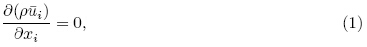
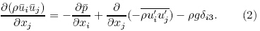
The equations shown here are for neutral conditions, where the buoyancy forces have been neglected.The variable ui is the component of velocity in i-direction(i= 1, 2, and 3 for directions x, y, and z, respectively),  is the turbulent flux, p is the ther-modynamic pressure, ρ is the density of the fluid, and g is the gravity acceleration.
The Reynolds decomposition introduces Reynoldsstress, which represents turbulence diffusive flux.The Boussinesq assumption, which states that theReynolds stress is linearly proportional to the rate ofstrains, is made here to define the turbulent flux:
where k is turbulence kinetic energy(TKE), μt is turbulence viscosity and would be yielded by solving auxiliary field equations of turbulence closure, which willbe discussed in Section 2.2.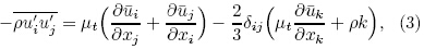
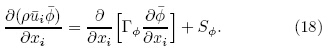
Gaseous substance is regarded as a passive scalar.The transport of a scalar can be modeled similarly.Turbulence transport of a scalar is taken to be proportional to the gradient of the mean value of the transported quantity. The unsteady-state form is applied here:
where C is the mass fraction or mass concentration ofa tracer,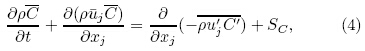
 is the turbulent flux of tracer, ΓC isthe turbulent diffusivity of tracer, and SC is the sourceof mass of tracer.
The turbulent diffusivity, ΓC, is expected fairlyclose to turbulence viscosity μt. The scale coefficientis defined as turbulent Schmidt number σC.
This assumption is known as the Reynolds analogy.2.2 Turbulence closure: the st and ard k-ε model
The turbulence closure scheme applied here iswidely used and can be referred to Launder and Spalding(1974).
The expression for the turbulence viscosity relatesto TKE, k, and dissipation rate ε:
where Cμ is a constant.
For conditions of stationary, neutral, and highReynolds number, the st and ard k-ε model equationsfor TKE, k, and dissipation rate ε are:
withwhere Gk is the production rate of TKE by shearstress, C1ε and C2ε are constants, σk and σε are turbulent Pr and tl numbers for k and ε respectively, and considered as constants too. Details about all these constants can be found in Launder and Spalding(1974).2.3 Wall boundary condition
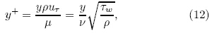
The above equations are used under highReynolds number condition and are invalid in the nearwall regions, where Reynolds number is low and viscous stresses dominate the flow. Instead, uniformshear stress is assumed and wall functions are usedin nodes adjacent to walls. Semi-empirical expressions(Launder and Spalding, 1974; Versteeg and Malalasekera, 2010)are used to relate to k, ε, and the frictionvelocity uτ.
The implementation of wall boundary conditionsin turbulence flow starts with the evaluation of twodimensionless parameters:
where uτ is friction velocity, Τw is the wall shear stress, μ and ν are dynamic viscosity and kinematic viscositycoefficients, respectively, and y denotes distance to the wall.
Considering the situation with y+ greater than11.63(Versteeg and Malalasekera, 2010), where thenodes adjacent to walls would be in the log-law regionof a turbulence boundary layer:
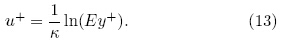
In this formula, κ is von Karman's constant(=0.4; Stull, 1988) and E is an integration constant. Forsmooth wall with constant shear stress, E has a valueof 9.793(Versteeg and Malalasekera, 2010).
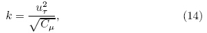
The expressions to relate k, ε, and friction velocity uτ are shown below:
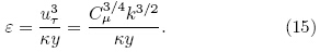
The expressions for wall shear stress Τw and production of TKE are given as:
3. Numerical method

All equations are discretized using the finitevolume approach. The spatial discretization of allequations has adopted the hybrid differencing schemeupon control volumes of non-uniform cuboid shapes.The fully implicit scheme is used for time integration of concentration field. These nonlinear equations are solved by an iterative method named SemiImplicit Method for Pressure-Linked Equations(SIMPLE). The brief description of SIMPLE algorithm isgiven below, and all detailed technologies except forthat about the control volumes of non-uniform cuboidshapes are explained in Versteeg and Malalasekera(2010), as well as Wang(2004).3.1 Finite volume method
Finite volume method is a special finite differenceformulation that is central to the most well-establishedCFD codes: CFD/ANSYS, FLUENT, PHOENICS, and STAR-CD(Versteeg and Malalasekera, 2010).This method is based on the conservation propertyof physical variables, which makes it much easier tounderst and than the finite element and spectral methods do. The key step of the finite volume method isthe integration of the transport equation over a three dimensional control volume.
The steady equations for RANS and st and ard k-εmodel can be derived from transport equation for ageneral property ∅:
Formal integration over a control volume gives
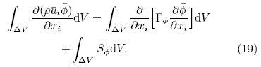
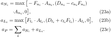
Figure 1 shows the schematic representation ofthe control volume adopted in our CFD model. Notation P denotes a general nodal point; notations Ni and Li denote neighbor of node P in positive and negativeidirection, respectively; notations ni and li denote side faces of control volume of node P in positive and negative i-direction, respectively; Δxi;P is referred to as control volume width in i-direction for node P; the distances between nodes P and Ni, and between nodes P and Li are identified by δxPNi and δxPLi respectively; similarly distances between point P and faceni, and between point P and face li are denoted byδxPni and δxPli, respectively.
 |
| Fig. 1. Schematic representation of the control volume. |
In the control volume shown in Fig. 1, Eq.(19)can be reformatted as
where A is the area of side face, and Sø is the averageof source strength in the control volume.3.2 Hybrid differencing scheme
In order to derive useful forms of the discretizedequations, the properties at the interface ni and li inEq.(20)are required. Many schemes can deal withthe interface properties, but the central differencingscheme seems a simple and reliable way of calculatinginterface values and the gradients because it uses linearapproximations and is second-order accurate. However, it would fail when convection is much strongerthan diffusion. The upwind scheme, which determinesthe interface values(not gradients)only by the upwind values, is another simple approach. Although itis absolutely stable, it has only first-order accuracy.To avoid these defects, we adopt the hybrid differencing scheme, a method that has combined advantagesof central and upwind differencing schemes.
Define convective mass flux F = ρu and diffusionconductance D = at the interface. We employ thecentral differencing approach to the diffusion term inEq.(20), no matter what scheme is used for convectiveterm. Equation(20)turns out to be:
In order to apply control volumes of non-uniformcuboid shapes, we deduce the discretized equationsfrom the uniform ones of Versteeg and Malalasekera(2010) and Wang(2004). We define the interpolationcoefficient as cni = and cli =
 for ni and li side faces, respectively.
Define non-dimensional cell Peclet number, Pe = , as a measure of the relative strength of convection and diffusion. The hybrid differencing scheme employsthe central differencing scheme when |Pe| < 1/c(cis interpolation coefficient defined above) and the upwind differencing when |Pe| > 1/c. The final steadytransport equation deduced with the finite volumemethod and hybrid differencing scheme is given as:
Here, it is noticed that the second column in theright side of Eq.(23)denotes the central differencingscheme.3.3 Fully implicit time scheme
The fully implicit scheme is used for time integration of the concentration field, because it is unconditionally stable for any length of the time step.
The unsteady form of transport equation integrated over a small interval Δt from t to t + Δt ina control volume is
The Semi-Implicit Method for Pressure-LinkedEquations(SIMPLE)is essentially a guess- and -correctprocedure for the calculation of pressure.
A pressure field p* is guessed to initiate theSIMPLE calculation process. Discretized momentumequations are solved using the guessed pressure fieldto yield velocity components ui* as follows:
Notice that Eq.(26)is obtained by replacingø with ui* and extracting the pressure gradient forcefrom the source term in Eq.(22). The variable Ai;P isarea of side face in i-direction, and bi;P is the remaining source term.
The guessed pressure field p* needs to be corrected. Define the correction p' as the difference between true pressure field p and the guessed pressurefield p*, so p = p* + p'. Similarly, define velocity correction ui', which satisfies ui = ui*+ui'.
The true fields p and ¹ui also satisfy the transportequation(Eq.(26)). Substitution of the transportequations of true field and guessed field yields the correction of velocity field:
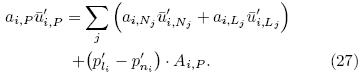
Equation(27)implies that the remaining sourceterm maintains the same between the true field and guessed field.
Since neglecting the term  (ai;Njui';Nj+ai;Ljui';Lj)would not change the final convergencevalue, SIMPLE algorithm omits these terms to simplify Eq.(27) and obtain the correction formula forguessed velocity field:

 .
.
To complete the correction, correction p' isneeded. The velocity field is also subject to the constraint of continuity equation, which replaces ø with number 1 and sets the source term to zero in Eq.(20)or Eq.(22). With ui = ui*+ui' and Eq.(28), theequation for p' can be deduced from continuity equation:
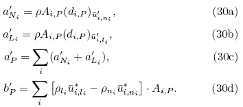
whereThe notation(di;P)ui'denotes the coefficient di;P of ui'when solving Eq.(28).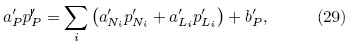
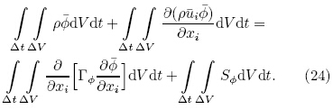
The whole iteration procedure of SIMPLE algorithm used in our model is given in Fig. 2.
 |
| Fig. 2. The SIMPLE algorithm. |
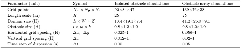
In order to validate the proposed numerical model, simulations of dispersion sources release, whichare expected to reproduce the wind tunnel experi-ments, have been carried out. Three datasets fromthe Compilation of Experimental Data for Validation of Microscale Dispersion Models(CEDVAL)provided by the Environmental Wind Tunnel Laboratory in University Hamburg are used in this study.The datasets are chosen because all the experimentswere well organized and clearly documented, and thedatasets are fully accessible at http://www.mi.unihamburg.de/Data-Sets.432.0.html. These wind tunnelexperiments were carried out at a scale of 1:200 in theBLASIUS wind tunnel at the Meteorological Instituteof the University of Hamburg. The first two corresponded to detailed measurements of the flow and dis-persion characteristics around an isolated rectangularobstacle, respectively, and the third one correspondedto array of obstacles. Dynamic similarity was maintained between simulations and wind tunnel experiments.4.1 Simulation setup
Urban areas with densely built-up l and use wouldsignificantly affect the local atmospheric condition, such as the airflow field and air quality, so it is necessary to evaluate the dynamic effects of buildings.On the other h and , for the purpose of validating anewly built numerical model, numerical simulationsfor simple cases are appropriate, because the factorswhich influence the experiments are fewer and easierto control and to evaluate. In this study, the first numerical validation case was performed for an isolatedrectangular obstacle.
The A1-1 and A1-5 data of CEDVAL were selected to validate the simulations of isolated obstacle.Although the A1-1 and A1-5 data belong to differentexperiments, they share the same experimental pa-rameters, including roughness length(= 7×10⁻⁴ m), friction velocity(= 0.377 m s-1), obstacle size(= 100mm×150 mm×125 mm) and so forth. The differencebetween these two datasets is the type of measureddata: the A1-1 dataset contains the measured data offlow characteristics and the A1-5 dataset contains themeasured data of dispersion.
In this case, two simulations were set up to correspond to A1-1 and A1-5 data, respectively. Thesesimulations applied the real scale(H=25 m). Table 1 and Fig. 3 show detailed parameters and aschematic representation of the computational domain and mesh used. The setup sketch of the single obstacle and sources is available at http://www.mi.unihamburg.de/fileadmin/files/forschung/techmet/physmod/cedval/datafiles/A1-5/A1-5-SS-1.GIF. The sources were released continuously and constantly. Because the concentration in this study is defined in adimensionless form, the source strength can be prescribed as any value and is omitted in this paper.The default turbulent Schmidt number for diffusionof tracer, σC, is set to 1, because of no implicationfor this value in measured data. The domain was extended up to a large distance in three directional axesto ensure that zero gradient assumption is rationalalong the lateral, outlet, and top boundaries. At theinlet boundary, velocity components ν(y-direction) and ω(z-direction)are considered to be equal to zero and the wind velocity and TKE profiles are providedaccording to the measured data.
 |
| Fig. 3. Schematic representation of isolated rectangular obstacle simulation domain:(a)mesh used for the computational simulations(the whole area is shown in the insert) and (b)positions of comparisons between simulation results and measured data. The points and lines indicate the positions for the validation in Section 4.2. |
The second case is considered for a little morecomplex situation with an array of obstacles, whichst and s for an extremely orderly city block. It is awell-organized group of buildings and also a commonelement in an urban area. Still this case is not too complex for the same reason. The B1-1 dataset ofCEDVAL, which contains measured data of both flow and dispersion, was selected to validate the simulationof array of obstacles. This dataset also shares the sameexperimental parameters and the same-size obstacles.The simulation setup adopted the same principle ofthe isolated rectangular obstacle simulation. Table 1 and Fig. 4 show detailed parameters and a schematicrepresentation of the computational domain and mesh, respectively. The 3×7 array of rectangular obstacles(Fig. 4)is applied in this simulation and the obstacleshave exactly the same dimension as that in simulationof isolated obstacle. The sources are set up at the leeward side of the building at origin(x=H=0, y=H=0), which is shown in the setup sketch of the sources.
 |
| Fig. 4. Schematic representation of the array of rectangular obstacles and the simulation domain:(a)mesh used for the computational simulations(the whole area is shown in the insert) and (b)positions of comparisons between simulation results and measured data. The points and lines indicate the positions for the validation in Section 4.3. |
Figure 5 shows the streamline of velocity aroundthe isolated obstacle. It is found that the mean flowimpinging the windward face of the obstacle is decelerated rapidly and part of the momentum in the maindirection is transferred to the spanwise and verticalmomentum. Streamline deflects and separates fromthe horizontal plane(Fig. 5b), and the flow is driveninto vertical downward and upward. The downwardpart creates a reverse flow extending to about 0.4Hin front of the lower half height of the obstacle(Fig. 5b), reattaches on its front face, and generates thehorseshoe vortex(Fig. 5b). The upward part flow separates at the sharp leading edge and then reattachesto the roof of the obstacle, and separates again at thedownwind edge(Fig. 5b). Similar behavior is alsofound at the sides of the obstacle(Fig. 5a). The separated flow passes over the building, and reattaches onthe ground further downwind at about 1.4H after theleeward side of the obstacle(Fig. 5b). The flow comesfrom the flow adjacent to the roof and lateral side ofthe obstacle travels upstream at the reattaching point and results in the formation of a recirculation regionbehind the obstacle(Figs. 5a and 5b).
 |
| Fig. 5. Computational streamline of isolated obstacle at(a)z/H = 0.5(plan view) and (b)y/H = 0(side view). |
The TKE field is given in Fig. 6. Values ofthe TKE close to corners of the building front wallsare the highest(Fig. 6b), which results from the extremely high wind velocity gradient. On the roof and the lateral sides of the obstacle, the TKE values arealso much higher than that of the free flow because ofthe high wind velocity gradients there. In the recirculation region, though the values of the TKE are not ashigh as that close to the corners, the values are higherthan those on the roof and side of the obstacle. In thedownstream region of recirculation, which is about 4Hafter the leeward side of the obstacle, the turbulencelevels are still slightly higher than those in the freeflow, which proves that the flow is still disturbed bythe obstacle.
 |
| Fig. 6. Computational TKE contours of isolated obstacle at(a)z/H = 0.5(plan view) and (b)(b)y/H = 0(side view). |
Comparison of the computed and measured velocity is shown in Fig. 7. The velocities are non-dimensionalized by the reference velocity at the height of 4H. The velocity profiles appear to be predicted reasonably well, especially in Figs. 7a and 7c-f. In Fig. 7b, the measured velocity adjacent to the roof is negative, while the computational velocity is not, whichindicates that the model under-predicts the separationintensity of the flow on the roof.
 |
| Fig. 7. Streamwise velocity from experimental data(unfilled circles) and simulation(filled circles and lines)of(a)A(x/H = {0.816, y/H = 0), (b)B(x/H = 0, y/H = 0), (c)C(x/H = 0.6, y/H = 0), (d)D(x/H = 0.84, y/H = 0), (e)E(x/H = 1.44, y/H = 0), and (f)F(x/H = 3.2, y/H = 0)in the case of an isolated obstacle. |
Comparison of the computed and measured TKEis given in Fig. 8. The data of velocity fluctuations inspanwise(y)direction at the center plane(y = 0)areunavailable in A1-1 dataset. The sum of velocity fluctuations in streamwise(x) and vertical(z)directionsinstead of complete TKE are used here. The Reynolds stress tensor in Eq.(3)is used to predict the velocityfluctuations. Although the general trend of predicted TKE is not as good as that of wind field, the shape and peak locations of the turbulence field are well predicted. At the location of long distance from the leeward side of the obstacle(Figs. 8e and 8f), the model predicts the TKE much better in both the shape and peak value. Figure 8b shows a large difference betweenthe measured peak value and the simulated one on theroof. The measured peak value is over three times asmuch as the simulated one. The reason may be theunderestimation of the velocity gradient due to underprediction of the separation intensity of the flow onthe roof(Fig. 7b).
 |
| Fig. 8. As in Fig. 7, but for velocity °uctuations. |
The concentration has been non-dimensionalizedby using the following equation:
where C is the mean concentration, Uref is the meanwind speed at reference height, which is 5.28H in thiscase, Cs is the tracer concentration in the sources, and Q is the total volumetric flow rate of the gassource.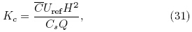
The concentration field after the time when itreaches equilibrium is chosen to validate.
In Sections 4.2 and 4.3, only experimental data(unfilled circles) and simulation with non-correctedturbulent Schmidt number(filled circles and solidlines)are used for discussion. The simulation withcorrected turbulent Schmidt number(dashed lines)will be discussed in Section 4.4 exclusively.
Comparison of the computed and measured concentration is shown in Figs. 9 and 10. Although the overall tendency of the model is to under-predict thespread and overestimate the peak values, the shape and peak locations are well predicted.
 |
| Fig. 9. Dimensionless concentration in spanwise(y)direction of line(a)LA1(x/H = 0.48), (b)LA2(x/H = 0.60), (c)LA3(x/H = 0.84), (d)LA4(x/H = 1.36), (e)LA5(x/H = 1.84), and (f)LA6(x/H = 3.2)at z/H = 0.08 in the case of an isolated obstacle. Results from the experimental data(unfilled circles), the simulation with non-corrected turbulent Schmidt number(solid curves with filled circles), and the simulation with corrected turbulent Schmidt number(dashed curves)are shown in each panel. |
 |
| Fig. 10. As in Fig. 9, but of line(a)LB1(x/H = 0.44), (b)LB2(x/H = 0.68), (c)LB3(x/H = 1.04), (d)LB4(x/H= 1.40), (e)LB5(x/H = 1.88), and (f)LB6(x/H = 3.60)at z/H = 0.28. |
The simulated wind fields are shown in Fig. 11.Even when an array of obstacles are present, generalcharacteristics of the wind field are quiet similar to those in Fig. 5 in the impinging region. The reverse region extends to about 0.2H in front of the first columnof obstacles(Fig. 11b). However, the recirculationregion shows something different. The recirculationregion extending to about 2.7H after the last columnof obstacles only appears after the middle row of theobstacles(Fig. 11a). The flow that wraps the lateral sides of the whole array only reattaches furtherdownwind and does not travel upstream to form a recirculating flow. Within the array of the obstacles, the velocity decreases as the column number of theobstacles increases(in the positive i-direction). Therecirculating flow appears in each region between anytwo obstacles in the streamwise(x)direction.
 |
| Fig. 11. Computational streamline around the array of obstacles at(a)z/H = 0.5(plan view) and (b)y/H = 0(side view) |
The simulated turbulence fields are shown in Fig. 12. The general turbulence field wrapping the wholearray of obstacles is also similar to that in Fig. 6.Within the array, the values of TKE maintain highlyclose to top corners of the obstacle front walls(Fig. 12b), although the values there decrease with the increasing column number. In the channel between two rows of obstacles and the recirculation region betweentwo columns(Fig. 12a), the values of TKE also decrease as the column number increases. Some valuesof TKE in the regions near the last column are evenlower than those in the free flow. This is due to thedecreasing of the wind velocity gradients caused by thereduction of wind velocity within the array along thestreamwise direction(Fig. 11).
 |
| Fig. 12. Computational TKE contours around the array of obstacles at(a)z/H = 0.5(plan view) and (b)y/H = 0(side view). |
Comparison of the simulated and measured velocity is shown in Fig. 13. The velocity field appearsto be predicted well in general. The prediction of thestreamwise velocity above the obstacle height H is better than that below it. At the center plane(Figs. 13a-c), prediction of the velocity underestimates the windspeed below about 0.3H, resulting in the underestima-tion of the intensity of the recirculation flow. At theplane of y/H = -1(Figs. 13d-f), the prediction turnsout to under-predict the wind speed below the obstacle height.
 |
| Fig. 13. Streamwise velocity from the experimental data(unfilled circles) and simulation(filled circles)of(a)A1(x/H= 0.56, y/H = 0), (b)B1(x/H = 0.8, y/H = 0), (c)C1(x/H = 1.04, y/H = 0), (d)A2(x/H = 0.56, y/H = {1), (e)B2(x/H = 0.8, y/H = {1), and (f)C2(x/H = 1.04, y/H = -1)in the case of an array of obstacles. |
Comparison of the simulated and measured TKEis shown in Fig. 14. Although the general predictionof TKE is not as good as that of wind field, the TKEfield shape and peak locations are also predicted rationally well. At the center plane(Figs.14a-c), themodel tends to under-predict the values of TKE belowthe obstacle height, while the simulation shows a beter agreement with the observation above that height.At the plane of y/H=-1(Figs.14d-f), the modelunder-predicts the entire TKE profiles, especially inthe region near surface.
 |
| Fig. 14. As in Fig. 13, but for TKE. |
Comparison of the simulated and measured con-centration is shown in Fig. 15. The concentration hasalso been non-dimensionalized by using Eq.(31). Theconcentration field shape and peak locations are alsowell predicted in the simulation. While the spread ofthe concentration field near leeward side(Figs. 15a and 15b)of the source building appears to be underpredicted, the peak value is over-predicted. In themiddle(Figs. 15c and 15d)of the source building and the building behind, both the spread and the peakvalues are under-predicted, while near windward side(Figs. 15e and 15f)of the building behind, the modelpredicted the concentration well both in the spread and peak values.
 |
| Fig. 15. Dimensionless concentration in spanwise(y)direction of line(a)L1(x/H = 0.52), (b)L2(x/H = 0.60), (c)L3(x/H = 0.76), (d)L4(x/H = 0.92), (e)L5(x/H = 1.08), and (f)L6(x/H = 1.16)at z/H = 0.06 in the case of an array of obstacles. Results from the experimental data(unfilled circles), the simulation with non-corrected turbulent Schmidt number(filled circles and solid curves), and the simulation with corrected turbulent Schmidt number(dashed curves)are shown in each panel. |
Clearly, the simulations have underestimated dispersal ability of the tracer. This may result from theimproper turbulent Schmidt number(σC= 1)for thetracer in the model. Flesch et al.(2002)reportedthat the turbulent Schmidt number could range from0.17 to 1.34. Other studies(Koeltzsch, 2000; Tomi-naga and Stathopoulos, 2007)also suggested differentvalues of turbulent Schmidt number in a large range.Therefore, it is necessary to determine a proper valuefor our simulations.
The correction used here is based on the measureddimensionless tracer concentration in the wind tunnel experiment and the simulation with non-correctedturbulent Schmidt number. The correction will be obtained by adopting some assumptions from the Gaussian plume model. It is emphasized hereby that: asmentioned in Section 1, the Gaussian plume model isnot comprehensive enough to be applied to an urbanarea; thus, our correction would not come from thearea that is strongly disturbed by the building. Thedetailed selections would be shown after the deductionof the correction factor.
Define the correction factor
where σCm is the corrected turbulent Schmidt number of tracer and σCs is the non-corrected turbulent Schmidt number of tracer.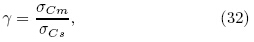
In the Gaussian plume model with Taylor's frozenturbulence hypothesis, the turbulent diffusivity can beobtained following the formula(Sykes and Gabruk, 1997)below:
where σy is the st and ard deviation of displacement oftracer in spanwise(y)direction.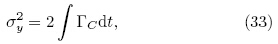
Combining Eq.(6)with Eq.(32), γ can berewritten as below:
where σys is the st and ard deviation of displacement ofsimulation and σym is the st and ard deviation of displacement of observational data.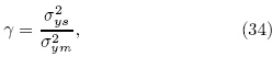
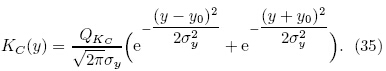
Figures 9 and 10 show that the simulations using the non-corrected dimensionless concentration inspanwise direction have a symmetrical shape with twopeaks. In this study, we assume that the dimensionlessconcentration in the region far enough from the areawhere the flow is strongly disturbed by the obstacle, corresponds to a Gaussian plume diffusion model as-sumption with two symmetrical point sources. Theformula is superposition of two symmetrical Gaussi and istributions:
This assumption of two sources is rational, because symmetrical recirculation regions shown in Fig. 5 tend to mix the tracer in each region and form two symmetrical sources.
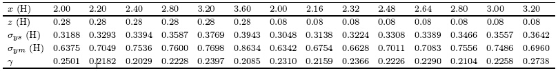
The correction factor was obtained from themeasured and simulated results of the isolated obstacle. In order to ensure the above Gaussianplume model's assumption can be satisfied as muchas possible, we avoided use of the data that camefrom the region strongly affected by the obsta-cle. Data beyond x/H= 2 seemed a reasonablechoice, since the region of x/H > 2 was after the recirculation region caused by the obstacle.The fitting values of σys and σym are shown inTable 2.
 |
In the present case, the average correction factorγ is 0.2277. This value is used to conduct anothersimulation of the isolated obstacle. The results arerepresented by dashed lines in Figs. 9 and 10. Thesimulation predicted the shape and spread much better. In the region close to the leeward side of the obstacle(Figs. 9a, 9b, 10a, and 10b), the simulation alsoshowed good prediction of the peak values. However, it underestimated the concentration in other regionsnot close to the leeward side of the obstacle(Figs. 9c-f and Figs. 10c-f).
The underestimation may have several reasons:1)the point source assumption, which does not exactly match the real condition because the recirculation region behind the obstacle is relatively broad; 2)the assumption of Gaussian-distributed concentrationin spanwise(y)direction, which implies homogeneousturbulent diffusivity(μt and ΓC)in the same direction, while Fig. 16 shows the heterogeneity of predicted turbulent diffusivity, which is obviously against the aboveassumption. It is also noted in Fig. 16 that the heterogeneity decreases as x/H increases, indicating thatthe choice of st and ard deviation of displacement inspanwise(y)direction from a much larger x may result in a better correction of turbulent Schmidt number. Unfortunately, no measured data were available at x/H > 3.6 in this dataset, which may need a futureinvestigation; 3)use of a constant turbulent Schmidtnumber as used in most CFD approaches, but manyinvestigations(e.g., Koeltzsch, 2000; Tominaga and Stathopoulos, 2007)indicated that turbulent Schmidtnumber is not a constant and depends on the localflow characteristics.
 |
| Fig. 16. Normalized turbulent diffusivity of momentum in spanwise(y)direction in the case of an isolated obstacle. Note: μtc is the turbulent diffusivity at y/H = 0. |
The corrected turbulent Schmidt number obtained above was also applied in another simulationfor the case of an array of obstacles, since they sharedthe same experimental parameters. The simulation generally predicted much better results in terms of boththe spread and the peak values, especially in the middle(Figs. 15c and 15d)of the source building and thebuilding behind. However, we still need to take thisresult carefully because of the underestimation of thepeak concentration in the isolated obstacle simulationwith corrected turbulent Schmidt number.5. Conclusions
A framework, based on a CFD approach solving steady-state RANS equations with the st and ardk-ε turbulence model, has been developed to simulate the flow, turbulence, and dispersion fields in urban builtup areas. Transport and dispersion modeling is made by solving an unsteady Eulerian transportequation using the velocity and turbulence field obtained from the steady RANS solution. The validationcompares simulated to measured velocity, turbulence, and dispersion fields for the neutral flow in a serieswind tunnel experiments conducted by Environmental Wind Tunnel Laboratory in University Hamburg.
It is found that the approach is able to predictthe velocity fields very well both above and below thebuilding height for the majority of simulated results.
The simulated TKE also corresponds to the measured one in both the shape and the location of thepeak, although the TKE values are not predicted asgood as those of wind velocity.
Without the correction of turbulent Schmidtnumber, the spread of simulated concentration fieldsis underestimated by the model. All peak values inspanwise(y)direction are overestimated in the simulation with an isolated obstacle, while in the case ofan array of obstacles, the peak values near the leeward side of the source obstacle are overestimated, but those in the middle of the source obstacle and theobstacle behind are underestimated. Both cases withthe correction of turbulent Schmidt number show abetter spread prediction, especially the array of obstacles case, while the prediction of the isolated obstaclecase underestimates the value of tracer concentrationin the areas far(x/H > 1)from the source obstacle.The imperfect point sources, heterogeneous turbulentdiffusivity, and the constant turbulent Schmidt as sumption used in the simulations may be responsiblefor the underestimation of the concentration spread.
Future work will focus on applying this CFD approach in real urban regions, as well as the applicationof more sophisticated turbulent closure, and a morecomprehensive treatment of the turbulent Schmidtnumber problem.
Acknowledgments: We would like to acknowledge the Environmental Wind Tunnel Laboratory inUniversity Hamburg for offering measured data on theInternet.
| Cheng, Y., F. S. Lien, E. Yee, et al., 2003: A comparison of large Eddy simulations with a standard k-ε Reynolds-averaged Navier-Stokes model for the prediction of a fully developed turbulent flow over a matrix of cubes. Journal of Wind Engineering and Industrial Aerodynamics, 91, 1301-1328. |
| Coirier, W. J., D. M. Fricker, M. Furmanczyk, et al., 2005: A computational fluid dynamics approach for urban area transport and dispersion modeling. Environmental Fluid Mechanics, 5(5), 443-479. |
| Davidson, M. J., W. H. Snyder, R. E. Lawson, et al., 1996: Wind tunnel simulations of plume dispersion through groups of obstacles. Atmos. Environ., 30(22), 3715-3731. |
| Di Sabatino, S., R. Buccolieri, B. Pulvirenti, et al., 2007: Simulations of pollutant dispersion within idealised urban-type geometries with CFD and integral models. Atmos. Environ., 41(37), 8316-8329. |
| Flesch, T. K., J. H. Prueger, and J. L. Hatfield, 2002: Turbulent Schmidt number from a tracer experiment. Agricultural and Forest Meteorology, 111(4), 299-307. |
| Gousseau, P., B. Blocken, T. Stathopoulos, et al., 2011: CFD simulation of near-field pollutant dispersion on a high-resolution grid: A case study by LES and RANS for a building group in downtown Montreal. Atmos. Environ., 45(2), 428-438. |
| Gromke, C., R. Buccolieri, S. Di Sabatino, et al., 2008: Dispersion study in a street canyon with tree planting by means of wind tunnel and numerical investigations-Evaluation of CFD data with experimental data. Atmos. Environ., 42(37), 8640-8650. |
| Hanna, S. R., M. J. Brown, F. E. Camelli, et al., 2006: Detailed simulations of atmospheric flow and dispersion in downtown Manhattan: An application of five computational fluid dynamics models. Bull. Amer. Meteor. Soc., 87(12), 1713-1726. |
| Higson, H. L., R. F. Griffiths, C. D. Jones, et al., 1995: Effect of atmospheric stability on concentration fluctuations and wake retention times for dispersion in the vicinity of an isolated building. Environmetrics, 6(6), 571-581. |
| Koeltzsch, K., 2000: The height dependence of the turbulent Schmidt number within the boundary layer. Atmos. Environ., 34(7), 1147-1151. |
| Krüs, H. W., J. O. Haanstra, R. van der Ham, et al., 2003: Numerical simulations of wind measurements at Amsterdam Airport Schiphol. Journal of Wind Engineering and Industrial Aerodynamics, 91(10), 1215-1223. |
| Launder, B. E., and D. B. Spalding, 1974: The numerical computation of turbulent flows. Computer Methods in Applied Mechanics and Engineering, 3(2), 269-289. |
| Li, X. X., C. H. Liu, D. Y. C. Leung, et al., 2006: Recent progress in CFD modeling of wind field and pollutant transport in street canyons. Atmos. Environ., 40(29), 5640-5658. |
| Macdonald, R. W., R. F. Griffiths, and S. C. Cheah, 1997: Field experiments of dispersion through regular arrays of cubic structures. Atmos. Environ., 31(6), 783-795. |
| —-, —-, and D. J. Hall, 1998: A comparison of results from scaled field and wind tunnel modeling of dispersion in arrays of obstacles. Atmos. Environ., 32(22), 3845-3862. |
| Mavroidis, I., 2000: Velocity and concentration measurements within arrays of obstacles. Global Nest: the Int. J., 2(1), 109-117. |
| —-, R. F. Griffiths, and D. J. Hall, 2003: Field and wind tunnel investigations of plume dispersion around single surface obstacles. Atmos. Environ., 37(21), 2903-2918. |
| —-, S. Andronopoulos, J. G. Bartzis, et al., 2007: Atmospheric dispersion in the presence of a three-dimensional cubical obstacle: Modeling of mean concentration and concentration fluctuations. Atmos. Environ., 41(13), 2740-2756. |
| Nozawa, K., and T. Tamura, 2002: Large eddy simulation of the flow around a low-rise building immersed in a rough-wall turbulent boundary layer. Journal of Wind Engineering and Industrial Aerodynamics, 90(10), 1151-1162. |
| Riddle, A., D. Carruthers, A. Sharpe, et al., 2004: Comparisons between FLUENT and ADMS for atmospheric dispersion modeling. Atmos. Environ., 38(7), 1029-1038. |
| Santos, J. M., N. C. Reis, E. V. Goulart, et al., 2009: Numerical simulation of flow and dispersion around an isolated cubical building: The effect of the atmospheric stratification. Atmos. Environ., 43(34), 5484-5492. |
| Solazzo, E., S. Vardoulakis, and X. M. Cai, 2011: A novel methodology for interpreting air quality measurements from urban streets using CFD modeling. Atmos. Environ., 45(29), 5230-5239. |
| Stull, R. B., 1988: An Introduction to Boundary Layer Meteorology. Kluwer Academic Publishers, 181 pp. Sykes, R. I., and R. S. Gabruk, 1997: A second-order closure model for the effect of averaging time on turbulent plume dispersion. J. Appl. Meteor., 36(8), 1038-1045. |
| Tewari, M., H. Kusaka, F. Chen, et al., 2010: Impact of coupling a microscale computational fluid dynamics model with a mesoscale model on urban scale contaminant transport and dispersion. Atmos. Res., 96(4), 656-664. |
| Tominaga, Y., and T. Stathopoulos, 2007: Turbulent Schmidt numbers for CFD analysis with various types of flowfield. Atmos. Environ., 41(37), 8091-8099. |
| Versteeg, H. K., and W. Malalasekera, 2010: An Introduction to Computational Fluid Dynamics: The Finite Volume Method. World Publishing Corporation, 151-280. |
| Wang Fujun, 2004: The Analysis of Computational Fluid Dynamics-The Theory and Application of CFD Software. Tsinghua Press, Beijing, 36-83. (in Chinese) |