 2013, Vol. 27
The Chinese Meteorological Society
Article Information
- XUE Ming, DONG Jili. 2013.
- Assimilating Best Track Minimum Sea Level Pressure Data Together with Doppler Radar Data Using an Ensemble Kalman Filter for Hurricane Ike (2008) at a Cloud-Resolving Resolution
- J. Meteor. Res., 27(3): 379-399
- http://dx.doi.org/10.1007/s13351-013-0304-7
-
Article History
- Received November 7, 2012
- in final form January 18, 2013


2 School of Meteorology, University of Oklahoma, Norman, OK 73072, USA;
3 Key Laboratory for Mesoscale Severe Weather/Ministry of Education, and School of Atmospheric Science, Nanjing University, Nanjing 210093, China
With a 2-h total assimilation window length, the assimilation of MSLP data interpolated to 10-min intervals results in more balanced analyses with smaller subsequent forecast error growth and better intensity and track forecasts than when the data are assimilated every 60 minutes. Radar data are always assimilated at 10-min intervals.
For both intensity and track forecasts, assimilating MSLP only outperforms assimilating radar reflectivity (Z) only. For intensity forecast, assimilating MSLP at 10-min intervals outperforms radar radial wind (Vr) data (assimilated at 10-min intervals), but assimilating MSLP at 60-min intervals fails to beat Vr data. For track forecast, MSLP assimilation has a slightly (noticeably) larger positive impact than Vr (Z) data. When Vr or Z is combined with MSLP, both intensity and track forecasts are improved more than the assimilation of individual observation type.
When the total assimilation window length is reduced to 1 h or less, the assimilation of MSLP alone even at 10-min intervals produces poorer 18-h intensity forecasts than assimilating Vr only, indicating that many assimilation cycles are needed to establish balanced analyses when MSLP data alone are assimilated; this is due to the very limited pieces of information that MSLP data provide.
Although hurricane track forecasts have improvedsignificantly over the last two decades, hurricane intensityforecasting remains a significant challenge(Cangialosi and Franklin, 2011; Rappaport et al., 2009).The slow improvement in hurricane intensity forecastingis believed to be at least partly due to limitedability to initialize tropical cyclone(TC)vortices accuratelyin numerical models(Rogers et al., 2006).Convective-scale structures in TCs are believed tohave direct or indirect impact on TC intensity and track forecasts(Fovell et al., 2009, 2010; Houze et al., 2007; Wang, 2009).
Techniques for initializing TC vortices includevortex bogusing(e.g., Kurihara et al., 1998; Pu and Braun, 2001) and direct initialization of TC vortexby assimilating observations on the vortex scale. Recently, a number of studies have demonstrated reasonablesuccess in assimilating airborne or ground-basedradar data for initializing TCs, and these studies typicallyuse the three-dimensional variational(3DVAR)(e.g., Du et al., 2012; Pu et al., 2009; Zhao and Xue, 2009; Zhao and Jin, 2008)or ensemble Kalman filter(EnKF)(e.g., Dong and Xue, 2013; Weng and Zhang, 2012; Zhang et al., 2009)methods. While theEnKF method is a theoretically advanced method thatmakes use of flow-dependent background error covariancederived from a forecast ensemble, Dong and Xue(2013; DX12 hereafter)also found that when startingfrom the GFS(Global Forecast System)analysisbackground, it takes 5 to 6 EnKF cycles of 10-minintervals, assimilating full volume radial velocity and reflectivity data from two coastal Doppler radars, tobring the minimum central pressure of a category 3hurricane to within 5 hPa of the observed best trackvalue. Even with a total of 13 analysis cycles at 10min apart, the final minimum pressure error remainedat nearly 5 hPa. Often, the minimum central pressurein TCs is difficult to analyze accurately without directsurface pressure observations.
Best track minimum sea level pressure(MSLP)has been used as observational data and assimilatedinto numerical models to help improve the TC intensityanalysis in recent research studies. Hamill et al.(2011)assimilated the so-called TCVital observationsevery 6 h using EnKF in a global forecast model. Here, TCVital is a human-synthesized dataset including thebest track estimates of TC minimum central pressure and center location. Despite clearly better track forecastsof TCs in their study compared to operationalbenchmarks, the resolution of their global model wasinsufficient to accurately predict the TC intensities;in fact, it was difficult for the global model to maintainthe initially intense TCs initialized using TCVitaldata in their study. Torn and Hakim(2009) and Wuet al.(2010)assimilated hurricane positions in realdata studies. Torn(2010)also assimilated best trackTC position and MSLP data along with other conventionalobservations every 6 h in a mesoscale model ata 36-km horizontal grid spacing using EnKF, althoughthe study did not specifically evaluate the impact ofTC position and intensity observations. Earlier, in aproof of concept study, Chen and Snyder(2007)assimilatedvortex intensity in terms of maximum vorticityusing EnKF in a simple two-dimensional(2-D)barotropic model and found improvement to the vortexintensity and track analysis and forecast. So far, according to our knowledge, the TCVital type of datahas not been assimilated into a hurricane predictionmodel at a cloud-resolving resolution with or withoutradar data using EnKF. It remains an open questionas to the kind of impact one can achieve with TCVitaldata in such situations. Most recently, Zhao et al.(2012)performed an experiment assimilating MSLPdata into a convection-resolving model for a typhoon, in addition to ground-based radar data using a 3DVARmethod; the impact of the MSLP assimilation was lostvery quickly(in less than 1 h)in their study due tothe univariate nature of their analysis method — therewas no temperature analysis increment to balance thepressure increment in their analyses. Given the multivariatenature of the EnKF method, it is hoped thatEnKF can do a much better job in assimilating MSLPdata on the convective scale.
In this paper, the impact of assimilating MSLPdata into Hurricane Ike (2008) using EnKF is examined.The best track MSLP data are assimilated aloneor in addition to the Doppler radar data, with the configurationsof the EnKF radar assimilation being thesame as in DX12. The rest of this paper is organized asfollows. Section 2 introduces the model, observations, and EnKF experiment setup. The analysis increments and the change to the hurricane intensity during theanalysis cycles are presented and discussed in Section3. The impacts of MSLP assimilation on the intensity and track forecasts are discussed in Section 4. Resultsfrom several sensitivity experiments are discussed inSection 5, and a summary is provided in Section 6.2. The case, prediction model, observations, and EnKF experiment design2.1 Hurricane Ike and model configurations
Hurricane Ike (2008) is the third costliest l and fallinghurricane in the US history. It made l and fallnear Galveston, Texas at 0700 UTC 13 September2008. More details of Ike near its l and fall can be foundin DX12. This study focuses on the analyses and forecastsof Ike shortly before and after its l and fall.
The prediction model used in this study is theAdvanced Regional Prediction System(ARPS; Xue et al., 2000, 2003). The physical domain is defined by a515×515×53 grid with a 4-km horizontal grid spacing.A vertical grid stretching scheme with a hyperbolictangent function is used(Xue et al., 1995); the meanvertical grid spacing is 625 m and the minimum verticalspacing is 50 m at the surface. The Lin et al.(1983)ice microphysics scheme is used along with the 1.5-order TKE-based sub-grid-scale turbulence and PBLparameterizations. Details on these physics optionscan be found in Xue et al.(2001, 2003). Other detailson physics and computational options are the same asthose used in DX12.2.2 Observations
The best track MSLP data from the US NationalHurricane Center are assimilated between 0400 and 0600 UTC 13 September in the first set of experimentsat intervals of either 10 or 60 min(Table 1).MSLP data, including their values and locations, atsuch intervals are obtained through linear interpolationbetween times when best track observations areavailable. The observed MSLP values changed onlyslightly within the 2-h data assimilation(DA)window.Radar observations are assimilated alone or togetherwith the MSLP data in the experiments to investigatetheir relative impacts. As in DX12, radial wind(Vr)or reflectivity(Z)data from two coastal WSR-88D radars at Houston-Gavelston, Texas(KHGX) and Lake Charles, Louisiana(KLCH)are assimilated, alwaysat 10-min intervals in this study. Details on theradar observations and their assimilation can be foundin DX12.
 |
In this study, we treat the best track MSLP dataas regular sea level pressure observations located at thebest track vortex center location, similar to Hamill etal.(2011). A simple pressure reduction equation(Eq.(1)of Benjamin and Miller (1990)) is applied as theobservation operator for the sea level pressure:
where PSL is the sea level pressure, P0 and T0 are thepressure and temperature at the first model level abovethe surface, z is the height of the first model level, γ isthe environmental temperature lapse rate(taken as 9.8K km−1), g is the gravitational acceleration, and R isthe gas constant. A bi-linear horizontal interpolationis used to project the sea level pressure from the modelgrid onto the best track position. The observationalerror of MSLP in the human-synthesized TCVitaldataset can range from 0.75 to 2 hPa(Tong Mingjing, 2010, personal communication). In this study, theobservation error of MSLP is assumed to be 1 hPa, smaller than 2 hPa used in Hamill et al.(2011). Thechoice of the relatively small MSLP observation erroris partially based on the observation that the analyzedMSLP without MSLP data is always positively biased(i.e., the analyzed hurricane is too weak)in this case, and a smaller MSLP observation error is expected to“push” the minimum pressure closer to the best trackobservation. Also we note that frequent assimilationof time interpolated best track data has an effect thatis somewhat similar to the nudging method, where themodel state is “nudged” towards the observations oran analysis persistently over a time period. In ourcase, the model state is constrained by the best trackobservations at multiple time levels through EnKFdata assimilation. Such frequent assimilation and theassociated model adjustments during the assimilationcycles are expected to increase/accelerate the impactof the very limited number of MSLP data within arelatively short period of time. The model grid, theradar locations, and radar data coverage are shown inFig. 1, along with the best track from 0300 UTC 13to 0000 UTC 14 September.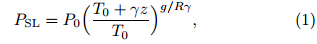
 |
| Fig. 1. The model grid, best track(denoted by blackdots), and radar coverage for Ike. The positions of tworadars are denoted by black squares. The range circlesof Houston-Gavelston, Texas(KHGX) and Lake Charles, Louisiana(KLCH)radars are for a maximum range of460 km. Best track covers 0300 UTC 13 to 0000 UTC14 September and hurricane locations are plotted every3 h. |
The ensemble square-root filter(EnSRF) ofWhitaker and Hamill(2002) forms the basis of ourEnKF assimilation system; the initial implementationof the EnSRF for the ARPS system is described in Xue et al.(2006) and the generation of ensemble initialconditions follows DX12.
Briefly, the forecast ensemble is created by addingmesoscale and convective-scale perturbations in twosteps. In the first step, a single 4-h forecast is runfrom the analysis at 1800 UTC 12 September of GFSof the National Centers for Environmental Prediction(NCEP)interpolated to the 4-km model grid;mesoscale perturbations are added to the 4-h forecastvalid at 2200 UTC in the entire model domain to createan ensemble of 32 members. The perturbations arecreated by smoothing Gaussian r and om perturbationswith zero mean using a 2-D recursive filter(Purser et al., 2003), with a horizontal de-correlation scale of 100km(e.g., Huang, 2000; Jung et al., 2012). The perturbationsare scaled to have st and ard deviations of 2m s−1 for u and v, 1 K for θ, and 1 hPa for p. For qv, the relative st and ard derivation is 10% of the unperturbedvalue, to avoid excessively large absolute perturbationsat the upper levels. Other state variablesare not perturbed in this step. Six-hour-long ensembleforecasts are then carried out from these perturbedinitial conditions to develop evolved background errorcovariance structures on the mesoscale.
In the second step, at 0400 UTC 13 September, additional convective-scale perturbations with asmaller horizontal de-correlation scale of 12 km and a vertical de-correlation scale of 4 km are added tothe ensemble forecast fields, but only in regions whereobserved Z exceeds 10 dBZ. These perturbations arecreated by applying a fifth-order-correlation smoothingfunction after Tong and Xue(2008). The st and arddeviations are 2 m s−1 for the wind components, 2 Kfor θ, 10% for qv, and 1 g kg−1 for all microphysicalvariables. These perturbations are found to yield bestanalysis and forecast results for the Ike case throughmany assimilation experiments in DX12 and are thereforeused here too.
The lateral boundary conditions are from the6-hourly operational GFS analyses with 3-hourly forecastsinterleaved in between, available on the 0.5degree grid. They are also perturbed by addingmesoscale perturbations created in the same way asin step one. Within ARPS, linear time interpolationsare performed between the boundary condition times.
In the first set of experiments(Table 1), MSLP and /or radar observations are assimilated in a 2-h windowfrom 0400 to 0600 UTC 13 September 2008, whichis the same as in DX12. After the assimilation, an18-h deterministic forecast is carried out from 0600UTC 13 to 0000 UTC 14 September from the ensemblemean analysis. In a control experiment(CNTL)used for reference, a forecast of the same length isstarted from GFS 0600 UTC analysis without any additionalradar or MSLP data. Schematics for threeexperiments, corresponding to VrP10W2h/ZP10W2h, VrP60W2h/ZP60W2h, and CNTL in Table 1, areshown in Fig. 2. Table 1 gives a full list of experiments.In the experiment names, letters Vr, Z, and P denote the assimilation of Vr, Z, and MSLP data, respectively. Numbers “10” and “60” following letterP in the names indicate the time interval(in minute)at which MSLP data are assimilated. The numberfollowing letter W denotes the total length of assimilationwindow in hour or minute. In all cases, radardata assimilation interval is 10 min. For example, inexperiment VrP10W30m, Vr and MSLP data are assimilatedtogether within a 30-min assimilation windowat 10-min intervals.
 |
| Fig. 2. Schematics showing the flowcharts for experiments that assimilate(a)radar and MSLP data every 10 minfor 2 h, (b)radar data every 10 min but MSLP data every 60 min for 2 h, and (c)reference forecast NoDA that doesnot assimilate any radar or MSLP data. The downward arrows denote MSLP DA times and the upward dashed arrowsdenote radar DA times. Ensemble forecasts are shown as thick horizontal arrows while single deterministic forecasts areshown as thin horizontal arrows. The ensemble DA experiments contain a 4-h single spin-up forecast period startingfrom GFS analysis at 1800 UTC 12 September 2008, which is followed by a 6-h ensemble spin-up period with mesoscaleperturbations added at 2200 UTC 12 September. Convective-scale perturbations are added at 0400 UTC 13 September, the beginning time of EnKF DA cycles. A single deterministic forecast starts from ensemble mean analysis at 0600 UTC13 September, the ending time of EnKF DA cycles. |
Covariance inflation and localization are appliedin the EnKF to alleviate the effects of sampling and other sources of error(e.g., model errors)within theensemble assimilation system. A horizontal covariancelocalization radius of 300 km is used for MSLP assimilation, chosen roughly based on the size of the backgroundvortex. Since there is only one MSLP observationat the analysis time and the MSLP is a vortexscaleparameter, a large horizontal localization radiusis reasonable to ensure that the impact of the MSLPassimilation extends to the entire vortex. A verticallocalization radius of 10 km for MSLP is determinedto be close to being optimal through a number of sensitivityexperiments; such a radius is reasonable becausethe surface pressure is directly linked to temperatureperturbations in the tropospheric air column.The localization radius for radar observationsis 12 km horizontally and 4 km vertically, as used inDX12 and is consistent with earlier studies of stormscaleEnKF radar data assimilation(Jung et al., 2008;Tong and Xue, 2008). Prior multiplicative covarianceinflation of 5% is applied to the state variableswithin the regions influenced(through EnKF updating)by the radar and /or MSLP data. Posterior additivecovariance inflation is applied to the state variablesin regions covered by assimilated radar observations;the magnitudes of the additive perturbationsare the same as those used in DX12. In experimentsassimilating both radar and MSLP, radar observationsare assimilated first, and MSLP data second. Thosestate variables having the strongest dynamic link tothe MSLP observation, including wind components, potential temperature, and pressure, are updated byMSLP. The updating of state variables by radar observations(Vr and /or Z)follows DX12. The reflectivitydata are used to update only pressure and the mixingratios of cloud water(qc), ice(qi), rain water(qr), snow(qs), and hail(qh)while the radial velocity dataupdate all of the eleven state variables, i.e., u, v, and w, potential temperature θ, p, mixing ratio of watervapor qv, and all microphysical variables. DX12 foundthat such settings yielded the best hurricane analysis and forecast.As found in DX12, whenever Vr is assimilated togetherwith Z, the analyses and forecasts are very similarto corresponding experiments assimilating Vr only.Thus, for brevity, the experiments assimilating both Vr and Z are not shown in this paper.3. Impact of MSLP observations on hurricane analysis3.1 Analysis increments
The wind and potential temperature analysis incrementsare plotted in Fig. 3 for P60W2h at 0500UTC 13 September, the first time that the MSLP dataare analyzed in this experiment; this is to illustrate theimpact of assimilating MSLP observation. The incrementis defined as the difference in the state variablesbefore and after the assimilation of MSLP observation.Figure 3 shows that after analyzing MSLP observation, a strong cyclonic circulation increment aroundthe MSLP data location(B in Fig. 3a)is evident at1 km above the mean sea level(MSL)(Fig. 3a), indicatingan enhancement to the background vortex thatis too weak. The center of the increment circulationis not co-located with the background vortex center, determined by the background MSLP(A in Fig. 3a), suggesting that the assimilation of MSLP observationis trying to change the vortex center location as well.The results suggest that the covariance between thepressure and wind fields derived from the ensemble isproviding important information to enable the MSLPdata to properly influence the wind fields in the EnKF, resulting in dynamically consistent multivariate analyses.A reduction in pressure is also noted at 1 kmabove MSL in the vortex region, as shown by the pressureincrement in Fig. 3a. The reduction is greaterthan 10 hPa above the MSLP location, and decreasesoutward.
 |
| Fig. 3. Increments of(a)horizontal wind component and pressure(every 200 Pa)at 1 km, (b)potential temperature(every 1 K)at 1 km, (c)vertical velocity w(every 0.2 m s−1)in the east-west cross-section along line CD in(a), and (d)potential temperature in the same vertical cross-section as(c), at 0500 UTC 13 September of experiment P60W2h. A and B denote the position of the background vortex center and the position of the MSLP observation, respectively. Thebackground wind vectors are also plotted in(c). |
The analysis increments of potential temperatureat 1 km above MSL are plotted in Fig. 3b. Whilethe potential temperature increment pattern is morecomplex than the pressure increment pattern, the incrementsare all positive in the vortex region, witha maximum value of about 5 K at this level, indicatingthat MSLP data assimilation has strengthened thewarm core of the cyclone. Positive increments of potentialtemperature extend upward to the mid troposphere, with an 1-K increment at the 5-km level abovethe MSLP data location(Fig. 3d). The 10-km verticallocalization radius used allows for the enhancementto the warm core in a deep layer. Increments ofwind, pressure, and potential temperature generallydecrease with height(figure omitted)as expected, butthey do reach the mid troposphere, indicating ratherdeep vertical correlation between surface pressure and these variables.
Vertical velocity(w)analysis increments, representingchanges in regions of updrafts and subsidenceare plotted along with the background wind vectors inFig. 3c, for a vertical cross-section through the forecastbackground vortex center(A in Fig. 3a) and theMSLP observation location(B in Fig. 3a). The positiveincrements of w reflect the enhancement of updraftsurrounding theMSLP location. Since the northwestquadrant of the vortex is already over the l and at this time and the vortex in that region has startedto weaken, the positive increments of w are broader and stronger on the southeast side(right of B in Fig. 3c). There is a region of negative increments insidethe eye(almost directly over B, the location of MSLPobservation), suppressing the weak updraft found inthe background vortex(as indicated by the wind vectors) and correctly establishing descending motion inthe eye region. The increments in temperature and wind fields are physically reasonable; they are consistentwith the fact that the background vortex is tooweak, and the decreased central pressure at 1-km altitudeby the MSLP data is accompanied by enhancedwarm core and eyewall updrafts as well as downwardmotion in the eye region.3.2 Impact of MSLP data on hurricane intensity during the analysis cycles
To investigate the impact of MSLP data on theanalyzed hurricane intensity during the assimilationprocess, the MSLP values of the analyzed hurricanebefore and after each analysis are plotted in Fig. 4.The best track MSLP data are linearly interpolated to10-min interval analysis times for comparison. In ourstudy, the MSLP value at each time is assimilated asa regular surface pressure observation located at thebest track vortex center, while the MSLP in the analysisis determined from the analyzed mean sea levelpressure field and this analyzed MSLP is not necessarilyat the best track vortex center.
We first examine the forecast and analysis MSLPswhen only MSLP data are assimilated. When MSLPobservations are assimilated at 60-min intervals inP60W2h over a 2-h window(at hours 1 and 2 intothe window), the analyzed MSLP decreases by about14 hPa, to 957 hPa, during the first analysis at 050013 UTC September(Fig. 4a). In the forecast over thenext hour without additional data assimilation, themodel MSLP increases to 964 hPa by 0600 UTC. Thesecond analysis of MSLP data at 0600 UTC reducesthe model MSLP to 954 hPa, 3 hPa higher than thebest track observation.
 |
| Fig. 4. The analyzed and forecast MSLP during the assimilation cycles of different experiments with(a)60-min and (b)10-min assimilation intervals for MSLP, compared to the best track. |
When MSLP is assimilated at 10-min intervalsin P10W2h, the analyzed MSLP is decreased by morethan 10 hPa during each of the first two analysis cycles(Fig. 4b). Over the 2-h assimilation window, the assimilation of MSLP always reduces the analyzedMSLP and the magnitude of reduction decreases graduallywith cycle as the model MSLP becomes closer tothe observed values. There is always an increase inMSLP in the ensuing forecast, but the amount of increasedecreases with the number of cycles, suggestingan increasing level of consistency among model statevariables as the model state is continually adjustedthrough the cycles. At 0520 UTC, the analyzed MSLPactually becomes about 2 hPa lower than the observedvalue interpolated to this time. Since the analyzedMSLP is not necessarily at the same position as theMSLP observation, this “over-correcting” behavior inP10W2h at 0520 UTC is possible because of unreliablespatial covariance causing under-shooting of analyzedpressure away from the MSLP data location. At theend of the assimilation window, the analyzed MSLP inP10W2h is almost exactly the same as the best trackvalue of roughly 951 hPa. Therefore, frequent assimilationof MSLP observations at 10-min intervals is ableto improve the intensity of the model TC in terms ofMSLP, making it approach the best track intensity after6 assimilation cycles.
Next, we examine the cases when Vr data are assimilatedalone, or together with MSLP data. In experimentVrW2h that assimilates Vr data only at 10-min intervals, the MSLP is reduced by about 5 hPa inthe first analysis at 0410 UTC, while in later cycles thedecrease by analysis is small and occasionally negative(e.g., at 0430 UTC). Much of the MSLP reduction isachieved during the forecast step in the earlier cycles, indicating that the model pressure field is adjustingto the improved wind field, not surprisingly becauseof the assimilation of a large number of Vr data(Fig. 4a). In VrP60W2h, the addition of MSLP observationat 0500 UTC further decreases the MSLP by about 1hPa compared to VrW2h(Fig. 4a), but the impact issmall in the ensuing cycles. At 0600 UTC, the secondassimilation of MSLP data results in a final analyzedMSLP in VrP60W2h that is about 2 hPa lower than inVrW2h. Therefore, the impact of assimilating MSLPdata at hourly intervals when Doppler radial velocitydata from two radars are assimilated at 10-min intervals, in terms of the analyzed MSLP, is minimal in thiscase.
In VrP10W2h, the MSLP data are also assimilatedat 10-min intervals together with Vr data, the analyzedMSLPs are always lower than those of VrW2h, and MSLP errors generally grow slower during theforecast step than in P10W2h(Fig. 4b). In VrW2h, the surface pressure reduction is achieved almost entirelythrough model adjustment while in VrP10W2h, the assimilation of MSLP provides direct help, resultingin much faster pressure reduction and more accuratefinal analysis of MSLP(Fig. 4b). In P10W2h, while the MSLP is reduced similarly as in VrP10W2h, the error growth is much larger in the forecast steps, especially during the earlier cycles; this is because ofthe larger mutual adjustments among the pressure, wind, and other state variables when no other directobservations are assimilated.
We now look at the cases when Z(instead ofVr)data are assimilated alone or together with MSLPdata. In experiment ZW2h, the model MSLP ischanged little by the Z assimilation before 0540 UTC(Fig. 4a). Reductions of 2 to 3 hPa in MSLP areachieved in the last three analysis cycles, likely a resultof improved cross-covariance between the microphysical and pressure fields in the ensemble(as discussedin DX12). In ZP60W2h, MSLP is assimilatedat 0500 and 0600 UTC; at 0500 UTC, an additionalMSLP reduction of 14 hPa is achieved by assimilatingMSLP data(Fig. 4a). While the storm weakensquickly to approximately 963 hPa in MSLP during thesubsequent 10-min forecast, the MSLP in the forecastis much lower than that of ZW2h, and remains so untilthe end of the assimilation window. Between 0510 and 0600 UTC, the assimilation of Z data every 10min causes very little change to MSLP, and it remainsmore or less constant; at 0600 UTC, the second analysisof MSLP data further reduces the minimum pressureby 10 hPa to reach 953 hPa, only 3 hPa higherthan the observed. Still, relatively rapid error growthin the subsequent forecast is expected with the verylimited number of MSLP analysis cycles in this case;this fact will be discussed further later.
The MSLP values in ZP10W2h are very similarto those of P10W2h before 0450 UTC(Fig. 4b). Inthe last few cycles, the analyzed MSLP in ZP10W2his closer to that of best track, and slightly higher thanthat of P10W2h. Comparing ZP10W2h and P10W2hindicates that the assimilation of Z in addition toMSLP does not seem to further improve the intensityanalysis. During some of the cycles(e.g., 0450–0530UTC), the analysis and forecast MSLP in ZP10W2hare slightly worse than P10W2h while in some othercycles(e.g., 0520 UTC), P10W2h over-analyzes theintensity somewhat. But in general, the assimilationof MSLP data every 10 min with and without Z dataresults in analyzed MSLP values that are close to thebest track data after several analysis cycles(Fig. 4b).Given the apparent effectiveness of MSLP data in analyzingthe minimum surface pressure of a hurricane, does it mean that we no longer need radar or othertypes of high-resolution observations? We will examinethe analyzed hurricane structures next, which willhelp answer this question.3.3 Analyzed hurricane structures
Figure 5 shows the wind, sea level pressure, and temperature fields of GFS analysis, and the finalEnKF analyses of VrW2h, P10W2h, and VrP10W2hat the surface and in the west-east vertical crosssectionsthrough the individual vortex center of eachexperiment. For brevity, only experiments with MSLPassimilated every 10 min are shown here. With Vr datafrom two coastal radars assimilated, the hurricane inVrW2h(Figs. 5c and 5d)is much stronger than thatin the GFS analysis(Figs. 5a and 5b), with both lowercenter pressure and larger radial pressure gradient. Inall three DA experiments, and in the GFS analysis, themaximum wind is always on the east side of the vortex.The vortex of VrW2h is much deeper than thatof the GFS analysis, as shown by the strong wind exceeding48 m s−1 extending to 6.4 km vertically(Fig. 5d). The maximum wind in VrW2h is approximately59.5 m s−1, which is much larger than the 44.5 m s−1in GFS analysis. The warm core is also much stronger and deeper in VrW2h than in the GFS analysis. WhenZ is assimilated in ZW2h, the final analyzed storm isalso stronger than in the GFS analysis, but weakerthan in P10W2h(figure omitted here; cf. DX12 Figs.6b, 6f, and 6j).
 |
| Fig. 5. The analyzed surface horizontal wind speed(shaded) and sea level pressure at 0600 UTC 13 September from(a)GFS analysis, (c)VrW2h, (e)P10W2h, and (g)VrP10W2h.(b), (d), (f), and (h)show the east-west cross-section ofhorizontal wind and temperature through the individual vortex center of each experiment. |
 |
| Fig. 6. Azimuthally averaged radius-height plots of horizontal winds from(a)GFS analysis, (c)VrW2h, (e)P10W2h, and (g)VrP10W2h.(b), (d), (f), and (h)show the radius-height plots of temperature anomaly of each experiment. |
In P10W2h, the minimum central pressure is evenlower than in VrW2h(Fig. 5e). The wind field ofP10W2h, having a maximum of 55.7 m s−1, is stronger and deeper than that of GFS analysis, but weaker thanthat of VrW2h(Fig. 5f). Strong winds of greater than48 m s−1 extend to around 3.6 km above the surfacein P10W2h(Fig. 5f), shallower than that in VrW2h(Fig. 5d). The warm core in P10W2h is stronger thanin the GFS analysis, but not as deep as in VrW2h. Itis clear that the assimilation of MSLP data is moreeffective in reducing the surface pressure while the assimilationof Vr data is more effective in establishingthe strong vortex circulation.
The analyzed minimum central pressure ofVrP10W2h is close to that of P10W2h and lower thanthat of VrW2h(Fig. 5g), and its vortex is stronger and deeper than in VrW2h with a maximum speed of61.7 m s−1 and the region with wind speed exceeding48 m s−1 extends to 7 km above the surface(Fig. 5h).The warm core in VrP10W2h is as deep as in VrW2h.In ZP10W2h, the final analysis is similar to P10W2h(figure omitted).
The right column of Fig. 5 also shows the temperaturefield in the vertical cross-sections. It is clearthat VrW2h(Fig. 5d) and VrP10W2h(Fig. 5h)producemore realistic warm-core temperature structuresthan in P10W2h(Fig. 5f); this is perhaps not toosurprising because MSLP data do not directly provideinformation on the vertical structures of the hurricane.In Fig. 5, the vortex structure in P10W2happears relatively smooth; by comparison, moreconvective-scale structures are analyzed when Vr observationsare assimilated and such convective-scalestructures can be important for hurricane prediction.The assimilation of MSLP does help strengthen thevortex although it tends not to introduce convectivescalestructures. When both types of observations areassimilated together, the hurricane acquires a lowercentral pressure and stronger and deeper vortex circulationsthan when Vr or MSLP is assimilated individually.
Individual cross-section shown earlier may not berepresentative of the vortex structure. Azimuthallyaveraged radius-height wind fields and temperatureanomalies of the final analysis at 0600 UTC are plottedin Fig. 6, together with those of the GFS analysis. Theazimuthal-mean horizontal winds in all three DA experimentsare substantially stronger than those in theGFS analysis. In P10W2h, the maximum azimuthalmeanwind exceeds 42 m s−1 while the maximum temperatureanomaly is over 12℃ and is located at 1–2 kmabove the surface(Figs. 6e and 6f). The latter verystrong temperature anomaly centered in the lower troposphereis not consistent with commonly observedor simulated structures within TCs(Emanuel, 2005;Wang, 2002)where the largest anomaly is usuallyfound in the mid-troposphere. With MSLP data beingthe only data source in this case, the vertical spreadingof observational information depends strongly onthe spatial error covariance, which tends to be less reliablethan direct observations; this may be the reasonfor the unrealistically-strong warm core at the low levelsfound in P10W2h. In VrW2h, the horizontal windfields have much larger horizontal gradients in the eyewallregion than in the GFS analysis, with roughly verticalisotachs in the eyewall and a maximum wind ofover 48 m s−1(Figs. 6c and 6d). The maximum temperatureanomaly is about 6℃ and is located at 6–8 kmabove the surface, a structure that is more consistentwith typical observed TC structures. In VrP10W2h, the structures of horizontal winds and temperatureanomaly are similar to those of VrW2h, except thatthe region with wind speeds exceeding 42 m s−1 isabout 2.5 km deeper than in VrW2h(Figs. 6g and 6h).In general, the assimilation of Vr and /or MSLP datasignificantly enhance the axisymmetric vortex circulation and warm core structure. The vortex structureobtained by assimilating Vr data is more realistic thanassimilating MSLP only and assimilating both Vr and MSLP data gives the strongest hurricane vortex.3.4 Sensitivity to model variable updating in EnKF
During the assimilation of MSLP, the model statevariables such as pressure, wind, and potential temperatureare updated. We examine here how the impactsof state variable updating evolve with time, which willhelp us underst and which model variables are mostimportant in maintaining the storm strength duringthe analysis-forecast cycles and how the model adjuststo the updated fields in the subsequent forecast.Towards this goal, a set of experiments is performedbased on experiment P60W2h. In these experiments, MSLP assimilation is performed at 0500 UTCusing the ensemble forecast background of P60W2h, but each experiment updates only a single or a subsetof state variables. A 20-min forecast is launchedfrom the ensemble mean analysis from each of theexperiments, which will be compared to the forecastlaunched from the ensemble mean forecast at0500 UTC, essentially from the forecast backgroundwithout further DA. The model variable updated byMSLP is indicated by the experiment name: ExpTonly updates potential temperature while ExpWTPupdates wind, potential temperature(θ), and pressure.The minimum value of surface pressure differencebetween the control forecast and the forecastswith MSLP DA(surface pressureforecast with DA minussurface pressureforecast without DA)is used as a pressureimpact index(PI)to measure the impact of DA on themodel surface pressure. A more negative PI indicatesa greater impact, i.e., the forecast storm is stronger.
The PIs of the experiments are plotted in Fig. 7at 0, 10, and 20 min after the DA time. At the initialtime(0500 UTC), the PIs of the experiments in whichpressure is updated by the MSLP data(ExpP, ExpTP, and ExpWTP)are all about –14.3 hPa, but are zeroin all other experiments(since the pressure is not updated).After 10 min, the large impact on pressurein ExpP decreases to –0.3 hPa, and to –0.15 hPa by20 min, indicating that the initial impact from MSLPDA is almost completely lost in this case. Clearly, updatingpressure only when assimilating MSLP data isineffective; this is consistent with the results of Zhao et al.(2012)where univariate analysis of the MSLPdata using the 3DVAR method was also found ineffective.
 |
| Fig. 7. Pressure impact index(PI; Pa)with time for experiments updating various model variables. |
The PIs of ExpW and ExpT increase from zeroat the initial time to –5.1 and –2.3 hPa, respectively, at 10 min of forecast, clearly due to the adjustment ofmodel pressure to the wind or potential temperaturefield updated by the MSLP data. Updating the modelwind field appears to have a larger impact than updatingθ on the forecast pressure. By 20 min, the PI ofExpW increases slightly(more negative)while that ofExpT decreases slightly, but the changes are less than1 hPa in both cases. Updating both wind and θ inExpWT leads to a more negative PI during the forecastthan updating wind or θ individually, giving PIsof –6.7 and –6.9 hPa at 10- and 20-min forecast times, respectively, and these values are very close to thoseof ExpWTP. At the same time, the PIs of ExpTP and ExpT are very similar at the corresponding times(Fig. 7)while the PIs of ExpWP(figure omitted)are verysimilar to those of ExpW. These results indicate thateven though MSLP contains pressure information, theupdating of wind and temperature fields when usingthe data is much more important than updating pressureitself; in fact, updating pressure itself has littleimpact on the subsequent forecasting with or withoutupdating other state variables; the improvement to theanalyzed MSLP is in a sense superficial in absence ofsupport of other state variables. In the model, thepressure field adjusts quickly to the temperature and wind fields, apparently through hydrostatic and gradientwind balance adjustments. Such results also pointto us the importance of cross-variable covariance derivedfrom the ensemble, which is responsible for theEnKF updating of state variables rather than pressurewhen assimilating the MSLP data.4. Impact on forecast4.1 Intensity forecast
The 18-h forecast MSLPs for all DA experimentsare plotted in Fig. 8, along with those of CNTL forecast, and they are compared to the best track data.The best track MSLP is 951 hPa at 0600 UTC 13September, one hour before l and fall; after l and fall, theMSLP gradually increases, and it is 980 hPa by 0000UTC 14 September(Fig. 8). Overall, all of the DAexperiments predict lower MSLPs than CNTL before1800 UTC. The slower weakening between 1500 and 2100 UTC compared to the best track might be a resultof model errors(DX12), leading to somewhat toostrong storms after 1800 UTC.
 |
| Fig. 8. Forecast(a, c)minimum sea level pressures and (b, d)surface maximum wind with time, compared to theobserved best track and CNTL. |
The MSLP of P60W2h at 0600 UTC is around955 hPa, slightly lower than that of VrW2h(Fig. 8a).However, the MSLP of P60W2h increases much fasterthan the best track and VrW2h during the first 3-hforecast, and is 5 hPa higher than VrW2h at 0900UTC. During the following forecast, the MSLPs ofP60W2h are always higher than those of VrW2h. TheMSLP of VrP60W2h is 2 hPa lower than that ofVrW2h at 0600 UTC, but becomes similar afterwards.When Z is assimilated in addition in ZP60W2h, thefinal analyzed MSLP is slightly lower than in P60W2hbut the predicted MSLPs become similar after 0900UTC.
With MSLP data assimilated every 10 min inP10W2h(Fig. 8c), the final analyzed MSLP is quiteclose to the best track. The predicted MSLP is similarto that of VrW2h after 0600 UTC, and is higher thanthe best track before 1800 UTC. All three experimentsassimilating MSLP at 10-min intervals are quite similarto one another, with differences in MSLP beingalways smaller than 2 hPa. Starting with a slightlyhigher MSLP than the other two at 0600 UTC, the intensityforecast of VrP10W2h during the 18-h forecastis generally the best among all the DA experimentsconducted in this study in terms of MSLP.
It appears that the assimilation of MSLP at 60-min intervals is insufficient to establish a strong and well-balanced hurricane. MSLP error in P60W2h increasesquickly during the first several forecast hours.More frequent MSLP assimilation at 10-min intervalsleads to a more balanced vortex and slower errorgrowth during subsequent forecast.
The assimilation of MSLP at 10- and 60-min intervalsin addition to Z data significantly improves theintensity forecast of ZW2h. Since the MSLP forecastof VrW2h is already close to the best track, frequentMSLP assimilation at 10-min intervals is necessary toachieve further noticeable improvement.
The maximum surface winds of forecasts in theexperiments are plotted in Figs. 8b and 8d, and arecompared to those of best track. At 0600 UTC, theanalyzed maximum winds of the experiments assimilatingradar and /or MSLP data are all stronger thanthose of CNTL, except that of ZW2h, which is similar.Experiments assimilating both Vr and MSLP(i.e., VrP60W2h in Fig. 8b and VrP10W2h in Fig. 8d)always have the strongest analyzed maximum wind, indicating the benefit of assimilating both Vr and MSLP observations. Although the analyzed maximumwinds in P10W2h and ZP10W2h are weakerthan those in P60W2h and ZP60W2h, respectively, the forecasts of P10W2h and ZP10W2h at 0900 UTCshow stronger winds than their counterparts assimilatingMSLP at 60-min intervals. This is more or lessconsistent with the MSLP forecasts, where the assimilationof MSLP at 10-min intervals helps to build upa more dynamically-balanced vortex, and the impactfrom DA lasts longer than when MSLP is assimilatedat 60-min intervals. Generally, the maximum surfacewind forecasts are close to one another in all experimentsafter 0900 UTC. Note that the maximum windcan be affected by localized convective activities whilethe MSLP tends to be a system-integrated more reliablemeasure of the vortex intensity(Zhu and Zhang, 2006).
In conclusion, with frequent assimilation of MSLPdata in a cloud-resolving model, hurricane intensityforecast can be improved; such improvement was notclearly achieved in Hamill et al.(2011)when assimilatingthe TCVital data into a coarser resolution globalmodel at a much lower frequency. The high assimilationfrequency is necessary to achieve sustained impacts.
MSLP assimilation at 10-min intervals outperformsVr assimilation in terms of the MSLP forecast.TheMSLP parameter measures mainly the overall vortexintensity, but does not necessarily represent wellsub-vortex convective-scale structures in a hurricane.For this reason, we further verify the wind forecasts ofCNTL, VrW2h, P10W2h, and VrP10W2h against theVr observations from the two coastal radars from 0600through 0900 UTC when Ike was near the coast. Theroot-mean-square differences(RMSD)between modelpredicted and observed Vr are plotted in Fig. 9. Suchcalculations are limited to regions where observed reflectivityexceeds 10 dBZ.
All DA experiments show clear improvement overCNTL when verified against Vr(Fig. 9). The RMSDagainst KHGX radar in CNTL grows rapidly partlybecause the vortex of CNTL moves slower than thebest track and other DA experiments from 0600 to0900 UTC(Fig. 10a). The RMSD values for VrW2hare 34% and 60% of those for P10W2h at 0600 UTCwhen verified against KHGX and KLCH radars, respectively(Fig. 9). The VrW2h analyses fit the observedVr data reasonably well, whereas the analyzedwinds assimilating MSLP data only match the observedVr data much worse. After 2 h of forecast, theRMSD values of VrW2h and P10W2h become closeras the RMSD of P10W2h decreases with time whilethat of VrW2h increases with time; their differencesare less than 1 m s−1 by 3 h for both radars. Theseindicate that wind errors are reduced during the forecastas the wind field adjusts to the improved vortexdue to MSLP DA, while wind errors that are reducedby the assimilation of Vr data increase as the forecasterror grows in general.
 |
| Fig. 9. Root-mean-square differences between observed and forecast Vr for experiments CNTL, VrW2h, P10W2h, and VrP10W2h, calculated against radar(a)KHGX and (b)KLCH. |
In a short range forecast(~3 h in our study), theassimilation of radar observations appears to have anadvantage over the assimilation of MSLP observationson the convective scale(as observed by radar data).Combining Vr and MSLP data clearly gives the best results.4.2 Track forecast
Figure 10 shows the predicted tracks, along withthe best track and average track errors, of 18-h forecastsfor selected experiments. The forecast vortexcenter positions are determined by the MSLP and areplotted every 3 h. Despite having a small initial positionerror of just 7 km, CNTL follows the westernmosttrack during the 18-h forecast, diverging from all of theDA experiments and the best track(Fig. 10a). Thefinal analyzed vortex centers in the experiments assimilatingMSLP are generally closer to the best trackthan those of CNTL and the experiments assimilatingonly radar observations. The errors in P10W2h, VrP10W2h, and ZP10W2h are 4, 4, and 2.6 km, respectively, comparable to(or even smaller than)thehorizontal grid spacing of the model. During the 18-h forecast, the tracks of the experiments assimilatingMSLP are similar to each other, except for ZP10W2h, which follows a more westward path at 1800 UTC.
 |
| Fig. 10.(a)Forecast TC centers(determined by MSLPposition)every 3 h from 0600 UTC 13 to 0000 UTC 14September(note that the map is stretched to highlight thedifference between the tracks).(b)18-h average track errors.The average track error of CNTL is 40 km and notshown here. |
Averaged over the 18-h forecast period, the trackerrors of P60W2h and P10W2h are generally comparableto those of VrW2h(Fig. 10b); the mean errorof P60W2h is 2 km larger than that of P10W2h.The track errors of all these three experiments aresignificantly smaller than the 41-km track error ofCNTL(not shown in Fig. 10b). The track errors ofVrP60W2h and VrP10W2h are both less than 10 km, smaller than the 12-km error of VrW2h. The trackerrors of ZP60W2h and ZP10W2h are only 60% of theerror of ZW2h. When MSLP is assimilated with radarobservations, the interval of MSLP assimilation(10 vs.60 min)does not have a strong impact on the track;the difference is always smaller than 1 km. In general, most of the experiments assimilating MSLP observationshave average track errors of less than 10 km.
Unlike intensity forecast, the track forecast appearsto be relatively insensitive to the MSLP assimilationinterval. This may be because the initial positionerrors can be quite effectively corrected in a few MSLPDA cycles, while intensity improvement requires morefrequent assimilation cycles to “nudge” and establisha well balanced vortex with sustainable intensity.5. Sensitivity of intensity forecast to assimilation window length
In the previous sections, we have shown that duringthe early analysis and forecast cycles, the MSLPerror grows much faster in P10W2h than in VrW2halthough the error growth rate decreases with time inP10W2h(Fig. 4). Clearly, many MSLP DA cycleshelp establish a more balanced vortex to slow downthe error growth in surface pressure. In this section, we further examine the impact of assimilation windowlength. Instead of the 2-h assimilation window used inprevious experiments, 1-h or 30-min assimilation windowis used, all ending at 0600 UTC, and all of themassimilate MSLP and /or Vr data at 10-min intervals.Figure 11 shows predicted MSLPs for the experimentsusing the three different window lengths, as comparedto the CNTL forecast and best track data.
 |
| Fig. 11. Forecast minimum sea level pressure from sensitivity experiments varying the assimilation window length, compared to the observed best track and CNTL. |
With a 30-min window in P10W30m, the analyzedMSLP at 0600 UTC is 953 hPa, close to the950 hPa of best track; it increases by 7 hPa in thefirst 3 h of forecast, the largest among all experiments(Fig. 11). In VrW30m, even though the final analyzedMSLP is about 3 hPa higher at 0600 UTC than that inP10W30m, the forecast MSLP at 0900 UTC is actuallya couple of hectopascals lower than in P10W30m, and remains lower throughout the 18-h forecast. Theassimilation of both MSLP and Vr in VrP10W30m resultsin a MSLP analysis of about 951 hPa, and theforecast values remain a few hectopascals lower thanthose in P10W30m and VrW30m, closer to the besttrack values; clearly, assimilating both Vr and MSLPdata gives better intensity forecasts than assimilatingone of them.
When the assimilation window is extended to 1h, the general behaviors of the three experiments aresimilar to the 30-min case, except that the MSLP errorsare further reduced by 1–3 hPa in the analyses and forecasts. In comparison, when a 2-h assimilation windowis used, P10W2h actually outperforms VrW2h, analyzing and predicting lower MSLPs that are in betteragreement with the best track. VrP10W2h performsslightly better than P10W2h in the MSLP forecast.
Compared to millions of Vr observations available, there is only one MSLP observation at each analysistime. The above results indicate that when usingtoo short assimilation windows, the assimilation of avery limited number of MSLP data is not able to establisha balanced storm as well as the millions of Vrobservations can, affecting the surface pressure prediction.The differences in the MSLP forecasts among thethree Vr assimilation experiments windows are muchsmaller, apparently due to the large number of Vr observations, while the forecasts assimilating MSLP dataare more sensitive to the window length(Fig. 11). Forthis particular case, 2 h appears sufficiently long forthe MSLP assimilation performed every 10 min to produceintensity forecasts comparable to assimilating Vrdata.
Assimilating both MSLP and Vr always outperformsthe assimilation of one of the observation types, regardless the window length. The improvement is larger for shorter windows.6. Summary and conclusions
Best track minimum sea level pressure(MSLP)data are treated as surface pressure measurements atTC vortex center and assimilated using an ensembleKalman filter(EnKF)at a convection-permitting resolution.The study was partly motivated by Hamillet al.(2011)who assimilated TCVital data, includingthe best track MSLP, into a global forecast modelusing EnKF; their results showed improved centralpressure analyses but the intensity forecast improvementwas quickly lost in the subsequent forecasts. Thelow assimilation frequency and coarse model resolutionwere believed to be the primary reason. In thisstudy, interpolated MSLP data are assimilated at 60-or 10-min intervals for a period of 30 min, 1 h, or 2 hfor Hurricane Ike (2008) before it made l and fall. Theassimilation and forecast experiments used the ARPSmodel and its EnKF DA system at a 4-km grid spacing.In addition, the relative impacts of MSLP versusthose of radar data are examined by assimilating radialvelocity Vr and /or reflectivity Z data from two coastaloperational radars individually or together with theMSLP data. The radar data are always assimilated at10-min intervals; the procedure for assimilating radardata using EnKF follows Dong and Xue(2012)exactly.
The first set of experiments examined MSLP DAover a 2-h window, at 60- or 10-min intervals. Theanalysis of MSLP is shown to enhance the hurricanecirculation and its warm core structure and it isachieved through cross-variable covariance estimatedby the EnKF. Through sensitivity experiments, it isshown that the updating of wind fields when assimilatingMSLP data has a more sustainable impact on theintensity forecast than updating temperature, whileupdating pressure by MSLP has little sustained impact;the model pressure tends to quickly respondto the wind and temperature fields through hydrostatic and gradient wind adjustments, not the otherway around. This further highlights the importanceof flow-dependent cross-covariance that allows for dynamicallyconsistent multi-variate analysis of the TCvortex.
The final analyzed TC vortex is shallower, and itsstructures are smoother when assimilating MSLP dataonly while radar data provide more convective-scalestructures; this is not surprising because the dense velocitydata contain much more convective-scale informationwhile the smaller covariance localization radiiused for radar data also help. The analyzed warmcore in the former case is also placed too low in theeye region. When MSLP and Vr data are assimilatedtogether, analyses that have better overall vortex intensity and convective-scale structures are obtained.
With 10-min assimilation intervals, the assimilationof MSLP data alone is able to keep the analyzedMSLP lower than that obtained by assimilatingVr data only, but the MSLP forecast error growth isfaster than the Vr case, apparently because of the adjustmentof the pressure field towards the less wellanalyzedwind and temperature fields. In the caseof Vr assimilation, the initially too high MSLP is decreasedduring the forecast periods, through pressureadjustment towards the better analyzed wind fields.The analyzed MSLP during the later cycles of the2-h assimilation window is very close to the best trackMSLP in the MSLP-assimilation case while that in theVr-only case remains a few hectopascals higher. Whenboth Vr and MSLP are assimilated, errors in both analyzed and forecast MSLPs remain very low in the latercycles.
A 60-min interval when assimilating the MSLPdata alone proves insufficient to establish a wellbalancedhurricane vortex in terms of MSLP forecast;the MSLP in the early forecast hours increases muchmore quickly than the best track(the hurricane wasweakening at this stage)while the MSLP error in theexperiment assimilating Vr data alone(at 10-min intervals)grows slower(even though the final analyzedMSLP had a slightly larger error). Again, combiningMSLP and Vr data has produced the lowest error inthe MSLP analysis and forecast. Assimilating reflectivitydata alone is able to reduce the MSLP error byonly one third in the final analysis relative to the noDA case.
Using 10-min MSLP assimilation intervals leadsto much better MSLP analyses and forecasts thanthat using 60-min intervals, resulting in lower finalMSLP analysis and reduced initial MSLP forecasterror growth, and outperforming the forecasts assimilatingVr or Z only. Assimilating MSLP in addition toZ data significantly improves the MSLP analysis and forecast but the improvement in addition to Vr datais much less, because the assimilation of Z data is notvery effective at decreasing the MSLP error.
The forecasts are also verified against Vr observationsfor the first 3-h forecast when Hurricane Ikeis near the coast. Not surprisingly, the much morevoluminous Vr data produce more convective-scalestructures than MSLP data and the improved fit ofthe forecast to Vr observations due to the assimilationof Vr data lasts throughout the 3-h forecast. The fit tothe Vr observations improves over time in the MSLPonlycase but the mis-fit remains slightly(about 0.5m s−1)larger than the Vr case by 3 h.
The assimilation of MSLP also improves the trackanalysis and forecast. Average 18-h track forecast errorswith MSLP assimilation are around 11–13 km, comparable to those obtained using Vr assimilation.Assimilation of MSLP together with Vr or Z improvestrack forecast more than the assimilation of Vr or Zonly.
Sensitivity of the intensity forecast to the lengthof the MSLP and /or Vr assimilation window is alsotested. Using shorter assimilation windows of 30 minor 1 h and 10-min assimilation intervals, MSLP forecastwith Vr assimilation outperforms the forecast withMSLP assimilation. Using a 2-h window, the oppositeis true. For shorter assimilation windows, combiningVr and MSLP gives even more benefits.
In summary, the assimilation of MSLP is able toimprove Hurricane Ike analyses and forecasts within acloud-resolving model, mostly through improvementsto the model wind and temperature fields, via crosscovarianceof surface pressure with wind and temperaturein the EnKF. Because of the very limited pieces ofinformation in the MSLP observations, frequent analysesare necessary to establish a balanced hurricanevortex having slow intensity error growth. Comparedto Vr data, MSLP data have less ability in producingconvective-scale structures(as verified against Vr observations) and the analyzed warm-core structure isnot very realistic. The best results are obtained whenVr and MSLP data are assimilated together.
In our case, the center position of Ike never deviatestoo far from the best track, and thus the assimilationof MSLP as a regular pressure observation locatedat the best track position is effective. Such treatmentcan be problematic if the simulated TC center is farfrom the best track. The assimilation of TC position and intensity separately(Torn, 2010; Wu et al., 2010)provides a possible solution to this problem.
In order to utilize ground-based radar data, weassimilated MSLP shortly before Ike made l and fall.For a rapidly intensifying TC over the ocean, theconclusion about the impact of MSLP assimilationmay differ. Further studies with more TCs that are invarious stages of development are needed to more completelyunderst and the impacts of MSLP assimilation.Other available observations should also be includedin the assimilation to obtain more comprehensive impacts.These can be topics for future studies.
Acknowledgments. Computations were performedin the National Institute of ComputationalSciences(NICS)at the University of Tennessee and in the Texas Advanced Computing Center(TACC)atthe University of Texas at Austin. Dr. Nathan Snookis thanked for proofreading the manuscript.
| [1] | Benjamin, S. G., and P. A. Miller, 1990: An alternative sea level pressure reduction and a statistical comparison of geostrophic wind estimates with observed surface winds. Mon. Wea. Rev., 118(10), 2099-2116. |
| [2] | Cangialosi, J. P., and J. L. Franklin, 2011: National Hurricane Center Forecast Verification Report, 77 pp. |
| [3] | Chen, Y. S., and C. Snyder, 2007: Assimilating vortex position with an ensemble Kalman filter. Mon. Wea. Rev., 135(5), 1828-1845. |
| [4] | Dong, J. L., and M. Xue, 2013: Assimilation of radial velocity and reflectivity data from coastal WSR-88D radars using an ensemble Kalman filter for the analysis and forecast of landfalling Hurricane Ike (2008). Quart. J. Roy. Meteor. Soc., 139(671), 467-487. |
| [5] | Du, N. Z., M. Xue, K. Zhao, et al., 2012: Impact of assimilating airborne Doppler radar velocity data using the ARPS 3DVAR on the analysis and prediction of Hurricane Ike (2008). J. Geophy. Res., 117, D18113, doi: 10.1029/2012JD017687. |
| [6] | Emanuel, K. A., 2005: Divine Wind: The History and Science of Hurricanes. Oxford University Press, Oxford, 296 pp. |
| [7] | Fovell, R. G., K. L. Corbosiero, and H. C. Kuo, 2009: Cloud microphysics impact on hurricane track as revealed in idealized experiments. J. Atmos. Sci., 66(6), 1764-1778. |
| [8] | —, —, A. Seifert, et al., 2010: Impact of cloud-radiative processes on hurricane track. Geoph. Res. Lett., 37, L07808, doi: 10.1029/2010GL042691. |
| [9] | Hamill, T. M., J. S. Whitaker, M. Fiorino, et al., 2011: Global ensemble predictions of 2009’s tropical cyclones initialized with an ensemble Kalman filter. Mon. Wea. Rev., 139(2), 668-688. |
| [10] | Houze, R. A., Jr., S. S. Chen, B. F. Smull, et al., 2007: Hurricane intensity and eyewall replacement. Science, 315(5816), 1235-1239. |
| [11] | Huang, X.-Y., 2000: Variational analysis using spatial filters. Mon. Wea. Rev., 128(7), 2588-2600. |
| [12] | Jung, Y. S., G. F. Zhang, and M. Xue, 2008: Assimilation of simulated polarimetric radar data for a convective storm using the ensemble Kalman filter. Part I: Observation operators for reflectivity and polarimetric variables. Mon. Wea. Rev., 136(6), 2228-2245. |
| [13] | —, M. Xue, and M. J. Tong, 2012: Ensemble Kalman filter analyses of the 2930 May 2004 Oklahoma tornadic thunderstorm using one-and two-moment bulk microphysics schemes, with verification against polarimetric radar data. Mon. Wea. Rev., 140(5), 1457-1475. |
| [14] | Kurihara, Y., R. E. Tuleya, and M. A. Bender, 1998: The GFDL hurricane prediction system and its performance in the 1995 hurricane season. Mon. Wea. Rev., 126(5), 1306-1322. |
| [15] | Lin, Y.-L., R. D. Farley, and H. D. Orville, 1983: Bulk parameterization of the snow field in a cloud model. J. Climate Appl. Meteor., 22(6), 1065-1092. |
| [16] | Pu, Z. X., and S. A. Braun, 2001: Evaluation of bogus vortex techniques with four-dimensional variational data assimilation. Mon. Wea. Rev., 129(8), 2023-2039. |
| [17] | —, X. L. Li, and J. Z. Sun, 2009: Impact of airborne Doppler radar data assimilation on the numerical simulation of intensity changes of Hurricane Dennis near a landfall. J. Atmos. Sci., 66(11), 3351-3365. |
| [18] | Purser, R. J., W.-S. Wu, D. F. Parrish, et al., 2003: Numerical aspects of the application of recursive filters to variational statistical analysis. Part I: Spatially homogeneous and isotropic Gaussian covariances. Mon. Wea. Rev., 131(8), 1524-1535. |
| [19] | Rappaport, E. N., J. L. Franklin, L. A. Avila, et al., 2009: Advances and challenges at the National Hurricane Center. Wea. Forecasting, 24(2), 395-419. |
| [20] | Rogers, R., S. Aberson, M. Black, et al., 2006: The intensity forecasting experiment: A NOAA multiyear field program for improving tropical cyclone intensity forecasts. Bull. Amer. Meteor. Soc., 87(11), 1523-1537. |
| [21] | Tong, M. J., and M. Xue, 2008: Simultaneous estimation of microphysical parameters and atmospheric state with simulated radar data and ensemble square root Kalman filter. Part I: Sensitivity analysis and parameter identifiability. Mon. Wea. Rev., 136(5), 1630-1648. |
| [22] | Torn, R. D., 2010: Performance of a mesoscale ensemble Kalman filter (EnKF) during the NOAA High-Resolution Hurricane Test. Mon. Wea. Rev., 138(12), 4375-4392. |
| [23] | —, and G. J. Hakim, 2009: Ensemble data assimilation applied to RAINEX observations of Hurricane Katrina (2005). Mon. Wea. Rev., 137(9), 2817-2829. |
| [24] | Wang, Y. Q., 2002: Vortex rossby waves in a numerically simulated tropical cyclone. Part I: Overall structure, potential vorticity, and kinetic energy budgets. J. Atmos. Sci., 59(7), 1213-1238. |
| [25] | —, 2009: How do outer spiral rainbands affect tropical cyclone structure and intensity? J. Atmos. Sci., 66(5), 1250-1273. |
| [26] | Weng, Y. H., and F. Q. Zhang, 2012: Assimilating airborne Doppler radar observations with an ensemble Kalman filter for convection-permitting hurricane initialization and prediction: Katrina (2005). Mon. Wea. Rev., 140(3), 841-859. |
| [27] | Whitaker, J. S., and T. M. Hamill, 2002: Ensemble data assimilation without perturbed observations. Mon. Wea. Rev., 130(7), 1913-1924. |
| [28] | Wu, C.-C., G.-Y. Lien, J.-H. Chen, et al., 2010: Assimilation of tropical cyclone track and structure based on the ensemble Kalman filter (EnKF). J. Atmos. Sci., 67(12), 3806-3822. |
| [29] | Xue, M., K. K. Droegemeier, V. Wong, et al., 1995: ARPS Version 4. 0 User’s Guide, 380 pp. Available at http://www.caps.ou.edu/ARPS. |
| [30] | —, —, and —, 2000: The Advanced Regional Prediction System (ARPS)A multi-scale nonhydrostatic atmospheric simulation and prediction model. Part I: Model dynamics and verification. Meteor. Atmos. Physics, 75(34), 161-193. |
| [31] | —, —, —, et al., 2001: The Advanced Regional Prediction System (ARPS)A multi-scale nonhydrostatic atmospheric simulation and prediction tool. Part II: Model physics and applications. Meteor. Atmos. Phys., 76(34), 143-165. |
| [32] | —, D.-H. Wang, J.-D. Gao, et al., 2003: The Advanced Regional Prediction System (ARPS), storm-scale numerical weather prediction and data assimilation. Meteor. Atmos. Phys., 82(14), 139-170. |
| [33] | —, M. J. Tong, and K. K. Droegemeier, 2006: An OSSE framework based on the ensemble square root Kalman filter for evaluating the impact of data from radar networks on thunderstorm analysis and forecasting. J. Atmos. Ocean Tech., 23(1), 46-66. |
| [34] | Zhang, F. Q., Y. H. Weng, J. A. Sippel, et al., 2009: Cloud-resolving hurricane initialization and prediction through assimilation of Doppler radar observations with an ensemble Kalman filter. Mon. Wea. Rev., 137(7), 2105-2125. |
| [35] | Zhao, K., and M. Xue, 2009: Assimilation of coastal Doppler radar data with the ARPS 3DVAR and cloud analysis for the prediction of Hurricane Ike (2008). Geophys. Res. Lett., 36(12), L12803. |
| [36] | —, X. F. Li, M. Xue, et al., 2012: Short-term forecasting through intermittent assimilation of data from Taiwan Region and Mainland China coastal radars for Typhoon Meranti (2010) at landfall. J. Geophy. Res., 117, D06108, doi: 10.1029/2011JD017109. |
| [37] | Zhao, Q. Y., and Y. Jin, 2008: High-resolution radar data assimilation for Hurricane Isabel (2003) at landfall. Bull. Amer. Meteor. Soc., 89(9), 1355-1372. |
| [38] | Zhu, T., and D.-L. Zhang, 2006: Numerical simulation of Hurricane Bonnie (1998). Part II: Sensitivity to varying cloud microphysical processes. J. Atmos. Sci., 63(1), 109-126. |