 2013, Vol. 27
The Chinese Meteorological Society
Article Information
- ZHONG Wei, WU Rongsheng. 2013.
- Newtonian Jerky Dynamics and Inertial Instability
- J. Meteor. Res., 27(3): 400-414
- http://dx.doi.org/10.1007/s13351-013-0311-8
-
Article History
- Received November 21, 2012
- in final form March 11, 2013


2 Institute of Meteorology and Oceanography, PLA University of Science and Technology, Nanjing 211101
Numerical analysis is used to derive time series of position, velocity, and acceleration under different sets of parameters, as well as their trajectories in phase space. The time evolution of kinematic variables indicates that a regular wave-like change in acceleration corresponds to steady wave-like variations in position and velocity, while a rapid growth in acceleration (caused by a rapid intensification in the force acting on the parcel) corresponds to track shifts and abrupt changes in direction. Stable limiting cases under the f-and β-plane approximations yield periodic wave-like solutions, while unstable limiting cases yield exponential growth in all variables. Perturbing the value of absolute vorticity at the initial position (ξ0) results in significant changes in the stability and dynamic features of the motion. Enhancement of the nonlinear term may cause chaotic behavior to emerge, suggesting a limit to the predictability of inertial motion.
The concepts of the distance,velocity(the firsttime derivative of distance), and acceleration(thesecond time derivative of distance)vectors are ofparamount importance in underst and ing particle kinematics.Newton’s second law formulates particlemovements according to dynamical concepts such asforce,momentum, and energy. The time derivativeof acceleration(i.e.,the third time derivative of distance),which is called jerk,attracted very little interestbefore the 1970s. Schot(1978)comprehensivelyreviewed the concept of jerk and its practical applicationsfor designing intermittent-motion and transitioncurves.
Early dynamical research of jerk sometimes evenmisunderstood the concept. French(1971)concludedthat the basic dynamics of an object influenced bya specified force had no relationship with second- orhigher-order derivatives of velocity. However,Appell’sequations of motion and the concept of accelerationenergy that emerged at the end of the 20th centuryhighlighted the importance of the dynamics of variableaccelerated motion(Mei et al., 1991). Huang(1981)introduced jerk into the Chinese literature and proposedthe concept of force variability,which connectsjerk to the change of the force. In answer to the question“what is the simplest jerk function that gives chaos?” asked by Gottlieb(1996),Sprott(1997a)established the theory of jerky dynamics by transformingthree first-order ordinary differential equations(ODEs)into a third-order,one-dimensional,autonomousODE system, and promoted the applicationof this theory to chaos research. Linz(1997)investigatedthree restrictions on the jerk function to ensurethat jerky dynamics can be derived from classicalNewtonian equations,in the process formulating theNewtonian jerky dynamics(which expresses the explicitphysical meaning of jerky motion).
It is well known that the forces acting on an airparcel change with time and space in atmospheric dynamics.A momentum equation with constant forceis therefore unable to completely describe the complexevolution of the atmosphere. Sudden changesin weather systems are always associated with adjustmentsof the large-scale circulation and /or the redistributionof internal meteorological quantities in dynamics.These changes could equivalently be consideredas the variability of external and /or internal forces innature. The elementary equations of atmospheric motioncan be regularly transformed into a second-orderODE of velocity,which is essentially a jerk equation.This analysis suggests that Newtonian jerky dynamicshas promising applications in atmosphere science.
In this paper,we attempt to further underst and the nonlinear aspects of atmospheric motion usingNewtonian jerky dynamics. We propose this frameworkas an operative option for investigating the evolutionof the atmosphere under the actions of variableforces. Inertial instability is one of the most importantdynamical mechanisms in atmospheric science. Thismechanism has been widely studied in the context ofthe genesis and development of weather systems(e.g.Emanuel, 1979,1982). In Section 2,we review the definitionsof the jerk function and Newtonian jerky dynamics, and then apply Newtonian jerky dynamics tothe inertial motion. We obtain the criteria for inertialinstability in the context of the meridional gradient ofperturbation kinetic energy. We then present theoretical and numerical analyses of the nonlinear inertialmotion equation and its instability criteria in Sections3 and 4. The results are summarized in Section 5.2. The jerk function and inertial motion equations2.1 Definition of the jerk function
The jerk vector may be defined as
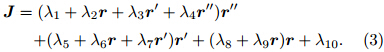
where a(t),V(t), and r(t)are functions of time(t), and indicate the acceleration,velocity, and distancevectors,respectively. The prime denotes the timederivative d/dt. In general,the jerky motion can bedetermined by a scalar real ordinary differential equationthat is(1)third-order,(2)explicit(i.e.,linear inthe highest derivative), and (3)autonomous(i.e.,notexplicitly dependent on time). This equation takes theformwhere r' and r' are the time derivative forms of velocity and acceleration,respectively, and J is the socalledjerky dynamics(Gottlieb,1996). Sprott(1997b)formulated the general second-degree polynomial jerkfunction asThe specific form of Eq.(3)is found by setting thecoefficients λ1–λ10 and identifying the dynamic characteristicsof the solutions. These dynamic characteristicsinclude motion under the action of variable forces and the possibility of chaos.

Not all jerky dynamics have explicit physicalmeaning. In the recognition,Linz(1997)defined Newtonianjerky dynamics as the subclass of all jerky dynamicsthat can be derived by taking the derivative ofa one-dimensional Newtonian equation with respectto time(Linz,1998). Newtonian jerky dynamics is relatedto the one-dimensional motion of a point particleof mass under the influence of an underlying force, and can be used to seek the physical relationships betweenthe motion and the variability of the force. Additionalrestrictions of Newtonian jerky dynamics are discussed by Linz(1997). Given a particle of constant mass macted upon by a complicated force vector F,the totaltime derivative of the Newton equation can be writtenas
As discussed by Linz(1997),three criteria for relatingthe jerk function to an underlying force should bemet:(1)the total and partial time derivatives of Fcannot explicitly depend on time;(2)terms that arequadratic(or even more nonlinear)in r" cannot enterinto the time-independent J; and (3)Schwarz’stheorem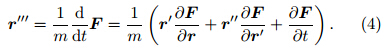
 must be satisfied to ensurethe integrability of J. Linz(1997)also examinedseveral famous nonlinear models,including thewell-known Lorenz model(Lorenz,1963)based on thesimplified form of the convection equations derived by Saltzman(1962).
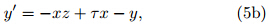
The original form of the model proposed by Lorenz(1963)is
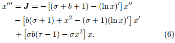
with σ,τ, and b representing control parameters.The jerk function can be obtained by the eliminationmethod asComparing Eq.(6)to Eq.(4),we find that the jerkfunction does not explicitly depend on time, and thereforefulfills criterion(1)above. However,Eq.(6)satisfiesneither criterion(2)nor criterion(3)due to thepresence of the logarithmic derivatives(ln x)' and theinequality between

 . This analysis shows that the Lorenz model is not Newtonian jerky.2.2 Equations for inertial motion
Inertial motion and its instability were first investigatedby Rayleigh(1916),who discussed atmosphericmotion under the co-action of the pressure gradient and Coriolis forces. The results of these fundamentalinvestigations have been widely used to explain thegenesis and enhancement of convection(e.g.,Tomas and Webster, 1997),the development of tropical cyclones(e.g.,Schubert and Hack, 1982), and the formationof secondary eyewalls(e.g.,Rozoff et al., 2012).The governing equations of inertial motion are fundamentallynonlinear,but most current tools for dynamicanalysis still rely on linearization. In this section,we apply Newtonian jerky dynamics to the twodimensionalequations of inertial motion to further ourunderst and ing of nonlinear atmospheric dynamics.
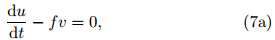
We assume that the basic flow is directed in thezonal direction,fulfills geostrophic balance, and is constantwith time. These assumptions mean that thegeostrophic velocity(ug,vg) and geopotential height(Φ)satisfy the equations ug = vg = 0, and
  = 0,where f is the Coriolis parameter(oftentaken as a constant f0 under the f-plane approximation).The equations of two-dimensional motion for aparcel in this flow are
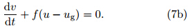
 Equation(7b)can then be written aswhere ζg = f−∂ug/∂y is the vertical component of thegeostrophic absolute vorticity. For an initial perturbationv0 > 0,the movement of the parcel at y0+δy canbe classified into three categories based on the value ofζg:(1)unstable motion(dv/dt > 0 with negative ζg);(2)stable oscillations(dv/dt < 0 with positive ζg); and (3)neutral states(ζg = 0 and dv/dt = 0). The same resultsare obtained for a southward displacement. This is classical dynamical analysis of inertial instability;however,this simple approach is only valid with thelinear approximation near y0 and the assumption that−fζLg is constant in Eq.(8). Here,we employ Newtonianjerky dynamics to investigate the more generalcase with complicated spatial structures of absolutevorticity and /or significant displacements in latitudes.
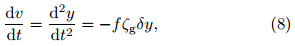
The kinematic meridional velocity and accelerationcan be defined as y' = v,y" = dv/dt = a. Substitutioninto Eqs.(7a) and (7b)yields the jerky functionfor inertial motion.
Two control parameters appear in Eq.(9). The parameterγ = β/f is the ratio of the meridional gradientof planetary vorticity to the value of planetaryvorticity, and can be thought of as representing theinfluence of the curvature of the earth on the inertialmotion. Two approximations may be made tosimplify the treatment: γ = 0(the f-plane approximation),or γ = β/f0,in which both β(= 10−11m−1 s−1) and f0(= 10−5 s−1)are set to be constants(the β-plane approximation). The parameterμ = f(∂ug/∂y−f)= −fζg represents the structure ofthe vertical component of geostrophic absolute vorticity,which reflects the structure of the underlying flow.Classical analysis of inertial motion typically assumesthat μ is constant. Here,we analyze the conditionsfor inertial instability associated with more complicatedmeridional distributions of ζg. Under the f- orβ-plane approximation,this parameter can be simplifiedto μ = −f0ζg. The dynamical features of Eq.(9)depend strongly on the control parameters γ and μ,or more specifically the meridional variability of planetary and absolute vorticity. Equation(9)satisfies thethree criteria outlined by Linz(1997). This jerk function,which is derived directly from the atmosphericmomentum equation,is therefore Newtonian jerky.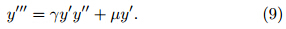
In typical classical analyses of inertial motion,theinitial conditions for the distance,velocity, and accelerationof the parcel satisfy
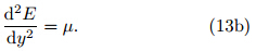
Since the acceleration y"=(d/dy)(y'2/2),the jerky″′ = y'(d2/dy2)(y'2/2). Given the additional conditionthat y' ≠ 0,the jerky function of Eq.(9)can bewritten aswhere E= y'2/2 is the zonal perturbation kinetic energy.The Newtonian jerky dynamics of inertial motionin the form of a third-order ODE that depends ontime is thereby transformed into a second-order ODEof the zonal perturbation kinetic energy equation thatdepends on position. We can then modify Eq.(10)toderive suitable initial conditions for Eq.(11):The criteria y" = dv/dt for estimating the instabilityof inertial motion then takes the equivalent formy" = dE/dy in Eq.(11). This means that the signof dE/dy determines the stability of the inertial motion.If dE/dy > 0,the zonal perturbation kineticenergy increases with meridional distance; the parcelis then unstable and accelerates away from its initialposition. By contrast,if dE/dy < 0,the parcel is stable and oscillates around its initial position. The keyto obtaining the dynamic features of the general equationsof inertial motion is therefore to seek the solutionof dE/dy under different sets of control parameters.3. Theoretical analysis


The simplified Newtonian jerky equation of zonalperturbation kinetic energy enables us to solve Eq.(11)theoretically. In this section,we use this approachto gain further insight into inertial stabilityunder more complicated control parameter regimes.3.1 Inertial motion under the f-plane approximation
Under the f-plane approximation,γ = 0 and Eqs.(9) and (11)can be simplified as
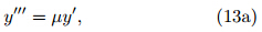
Equation(13)is linear if μ is a constant,yieldingthe criterion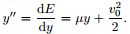 We follow theclassical analysis by assuming that the initial perturbationin the meridional direction y is positive(northward).The stability of the system is then determinedsolely by the sign of μ(an initial southward perturbationyields the same result). This result is identical tothat obtained from classical analysis of inertial instability:the system is stable when the absolute vorticityis negative(positive μ) and unstable when the absolutevorticity is positive(negative μ).
The dynamic features of this system change whenμ is defined as a function of y. We define μ as aquadratic polynomial with the form μ = c0+c1y+c2y2for simplicity,where c0,c1, and c2 are constants. AlthoughEq.(13b)still retains its linear features,Eq.(13a)has nonlinear terms when one(or both)of c1 and c2 is(are)non-zero. The meridional distributionof the absolute vorticity is determined by the choicesfor c0,c1, and c2. If c1 and /or c2 are/is non-zero,themeridional gradient in the absolute vorticity is nonzero and analogous to the β effect(Montgomery and Kallenbach, 1997). This difference leads to significantchanges in the dynamic behavior of the system.
For the sake of discussion,we define some of theparameters of the ambient flow based on the relationshipbetween μ and ζg. Specifically,we define themeridional gradient of absolute vorticity ζy = dζg/dyas −dμ/(f0dy),the second-order derivative of absolutevorticity ζyy = d2ζg/dy2 as −d2μ/(f0dy2),theabsolute vorticity at the initial position ζ0 = ζg|y=0as −(μ/f0)|y=0, and the meridional gradient of theinitial absolute vorticity ζy0 as −(dμ/f0dy)|y=0. Theconstants c0,c1, and c2 are given by
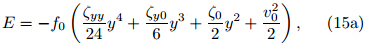
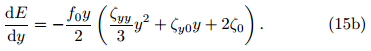
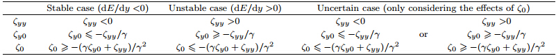
Substituting from Eqs.(14) and (12),the theoreticalsolutions of Eq.(13b)areEquation(15a)indicates that the system stateis determined not only by the structure of the ambientflow(ζyy,ζy0, and ζ0),but also by the meridionaldisplacement y. Table 1 lists the criteria for inertial instabilityassociated with various configurations of theflow parameters. If the meridional displacement y isassumed to be positive,then two limiting cases areobtained that are qualitatively independent of y. Thefirst case is that all of the flow parameters are positive(ζyy > 0,ζy0 > 0, and ζ0 > 0). This case resultsin stable motion(dE/dy < 0). In other words,if the(quadratic)absolute vorticity has a minimum, and theabsolute vorticity and its gradient are positive at theinitial position,then the motion is inertially stable.The second case is that all of the flow parameters arenegative(ζyy < 0,ζy0 < 0, and ζ0 < 0). This caseresults in unstable motion,meaning that the parcelwould accelerate away from its initial position. Outsideof these two limiting cases,the dynamic featuresare uncertain. All three parameters are determined bythe distribution of ζg,with ζyy and ζy0 dependent onthe shape of the distribution and ζ0 simply the valueof ζg at the initial position. The simplest approach isto retain the shape of ζg and change the sign of ζ0.In this case,dE/dy may change sign as y varies. InSection 4,we perform numerical calculations to showthe uncertainty in this condition.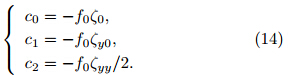

We primarily consider cases for which the flowparameters are non-zero,as these represent the mostcommon situation. If one or more of the flow parametersare zero,the distribution of absolute vorticitybecomes monotonic or constant. These cases can beconsidered by setting the relevant parameters to zero.
Taking the meridional structure of ζg into consideration,Eq.(13a)can be rewritten as
Equation(16)may then be compared with the simplestchaotic dissipative system described by Sprott(1997b). Although no y" term appears on the righth and side of Eq.(16),the nonlinear terms yy' and y2y'may generate chaos. The form of the solution is determinedby the parameters c0,c1, and c2,which correspondto the physical atmospheric parameters ζyy,ζy0, and ζ0.
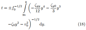
The expression of E in Eq.(15a)indicates thatthe paths in the y'−y phase plane are closed oval-typecurves:
The solution y(t)is then obtained implicitly as an inversefunction through the quadrature(omitted here), and the time period of the motion isWe can use Eq.(18)to investigate whether the phaseplane plots yielded by this system(Sprott,1997b)areperiod-1(limit cycle)orbits,period-doubling orbits,or chaotic orbits. The results of this investigation arepresented in Section 4.3.2 Inertial motion under the β-plane approximation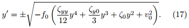
Changes in the Coriolis parameter must be takeninto account if the parcel is displaced a significant distance.In this case,we should employ the β-planeapproximation with a non-zero constant γ in Eqs.(9) and (11).
To recover the nonlinear term γy'y",we start withthe simple ambient flow described by a constant μ.
Usually γ = β/f0 > 0 and (eγy −1)> 0,in which casethe sign of dE/dy is determined solely by the sign of μas in the classical inertial instability analysis discussedabove. Furthermore,if both control parameters(μ and γ)are constants,the jerk function depends only on y' and y". This jerk function can then be written as asecond-order autonomous ODE in y', and cannot exhibitchaos(Gottlieb,1998).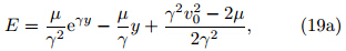
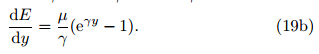
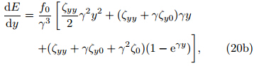
The theoretical solutions of Eq.(11)for the morecomplex ambient flow with μ = c0 + c1y + c2y2(withthe constants set as in Eq.(14))are
where(1 − eγy)< 0. The criteria for instability accordingto Eq.(20a)are listed in Table 2. A stablelimiting case results when ζyy <0,ζy0 ≤ −ζyy/γ, and ζ0≥ −(γζy0 + ζyy)/γ2. These three conditionsare equivalent to(1)the(quadratic)absolute vorticityhas a maximum in the direction of the initial displacement,(2)the meridional gradient of the absolutevorticity is less than |ζyy|/γ, and (3)the absolute vorticityat the initial position is positive and greater than|γζy0+ζyy|/γ2. An unstable limiting case results whennone of these three conditions is met. The stability orinstability of all other cases depends not only on thestructure of the ambient flow,but also on the meridionaldisplacement y. In Section 4,we provide numericalresults for cases in which the shape of the absolutevorticity distribution is retained while the sign of ζ0 ischanging.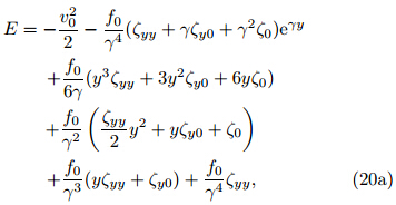
The preceding analysis indicates that inclusion orexclusion of the β effect does not affect the stabilityor dynamic features of inertial motion if the absolute vorticity distribution is constant; however,the nonlinearterm γy'y" exerts a significant influence on thestability criteria if the absolute vorticity varies in themeridional direction. Figure 1 shows the meridionalprofiles of ζg in stable and unstable cases under thef- and β-plane approximations. Under the f-planeapproximation,if ζg increases with a meridional displacementfrom a positive initial value,the system isinertially stable. By contrast,the system is inertiallyunstable if ζg decreases with a meridional displacementfrom a negative initial value. Under the β-planeapproximation,the ζyy criterion for stability(or instability)changes signs. The criteria for ζy0 and ζ0 aremore complicated,with threshold values that dependon the parameters ζyy,ζy0, and γ. The requirementsfor the stable and unstable limiting cases are quitestrict. Violation of any of the requirements shown inFig. 1(or listed in Tables 1 and 2)leads to uncertaintyin the inertial stability of the system. This uncertaintyis analyzed numerically in the next section.
 |
| Fig. 1. A sketch of the absolute vorticity(ζg)with meridional displacement(y)in the stable(solid line) and unstable(dashed line)cases under(a)the f-plane approximation and (b)the β-plane approximation. |
In this section,we calculate numerical solutionsto the Newtonian jerky equations that complementthe theoretical discussion in Section 3. The kinematicdefinitions of the perturbation meridional velocity(v) and acceleration(a)enable them to be expressed asdy/dt and d2y/dt2,respectively. The 3rd-order ODEfor the solitary variable y(Eq.(9))can be convertedto a group of closed ODEs for y,v, and a:
The parameter γ is set to either 0(under the f-planeapproximation)or a constant β/f0(under the β-planeapproximation). As in Section 3,the parameter μ isdefined as a second-order polynomial in y. This ensuresthat the equation of inertial motion is nonlineareven under the f-plane approximation. The numericalresults are obtained using the MatlabTM function ode45. The ordinary atmospheric momentum equationsbased on Newton’s second law consist of onlytwo equations: a kinematic equation defining the velocity and a dynamic equation describing the rate ofchange in this velocity under the influence of forces.This system cannot produce chaos because it only includesa two-dimensional phase space(Sprott,1997b).Gottlieb(1996)pointed out that Newtonian jerky dynamicsprovides a topological geometric foundation forestablishing the relationship between chaotic motion and variable forces.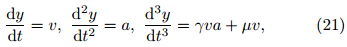
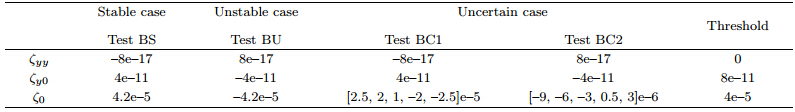
We have designed eight numerical experiments totest the stability of the flow under different sets ofparameters. The values of the parameters for each experimentare listed in Tables 3 and 4. The planetaryvorticity and its meridional gradient are approximatedas f0 = 10−5 s−1 and β = 10−11 m−1 s−1(β = 0 underthe f-plane approximation). We use the initialconditions set out in Eq.(10) and prescribe an initialnorthward perturbation velocity(v0)of 1 m s−1 at theinitial position y0 = 0. We use the criteria for the β-plane approximation to calculate the threshold valuesfor the parameters ζy0 and ζ0(Table 4).

The f-plane approximation is appropriate formesoscale or smaller scale atmospheric motions. Theparameter values listed in Table 3 are therefore specifiedto ensure an apparent and reasonable change in ζgwithin 200 km(Figs. 2a and 3a). The ambient flow,instability criteria, and time series of perturbations inthe stable(test FS) and unstable(test FU)limitingcases are shown in Figs. 2 and 3,respectively.
 |
| Fig. 2.(a)The meridional distributions of absolute vorticity(ζg; s−1) and the meridional gradient of perturbation kinetic energy(dE/dy).(b)The time series of distance(y; km),velocity(v; m s−1), and acceleration(a; m s−2)for test FS. |
 |
| Fig. 3. As in Fig. 2,but for test FU. |
The meridional gradient of perturbation kineticenergy dE/dy decreases monotonically toward thenorth in the stable case(Fig. 2). Each of the variabletime series follows a wave-like pattern with aperiod of approximately 100 h(~4 days). The timescale of these variations is consistent with the definitionof inertial waves. The meridional displacement ofthe parcel is limited to approximately 100 km in eitherdirection, and the magnitude of the perturbationvelocity is systematically less than the initial value.The evolution of the acceleration nicely illustrates theeffects of force variability on the motion. The fluctuationsin the acceleration are weak and wave-like, and oriented in the opposite direction to the fluctuationsin velocity. This result suggests that the forcevariability caused by the meridional variation of absolutevorticity acts as a restoring effect,generatingan oscillation of the air parcel. By contrast,all of thevariables increase dramatically with time in the unstablecase(positive dE/dy). Test FS shows that amonotonic northward increase in ζg results in stability,while test FU shows the monotonic decrease in ζgresults in instability. These results are consistent withthe classical analysis of inertial instability.
The dynamic features of the system are more complicatedif some of the criteria for the stable or unstablelimiting cases are not satisfied. We have designedtests FC1 and FC2 to more fully explore these uncertaincases under the f-plane approximation. Theparameters for these tests are listed in Table 3. Welimit ourselves to varying the value of ζ0 and investigatehow these cases differ from the stable and unstablelimiting cases. Each test comprises five memberswith different values of ζ0.The meridional distributions of ζg and dE/dy intest FC1(Fig. 4a)are nearly identical to those in testFS(Fig. 2a),except that the sign of ζg is differentat the initial position. However,the time series of thevariables have two new properties(Fig. 4b). First,thewave-like structure of the time series shows evidence ofmultiple periods. In particular,the acceleration spikesover a relatively short time in each cycle. This rapidgrowth in the acceleration is one order of magnitudegreater than the normal growth over such a short time(~10 h), and implies a rapid intensification in the forceacting on the air parcel. This intensification correspondsto a fast transition in the velocity from thenegative extreme to the positive peak. The largestsouthward displacement is nearly 400 km. The rapidintensification of the force significantly influences theparcel trajectory and the direction of motion.
 |
| Fig. 4. As in Fig. 2,but for test FC1. The colors correspond to ζ0 = –1×10⁻⁵ s−1(black),ζ0 = –1.5×10⁻⁵ s−1(red),ζ0 = –2×10⁻⁵ s−1(blue),ζ0 = –2.5×10⁻⁵ s−1(yellow), and ζ0 = –3×10⁻⁵ s−1(violet). |
Second,the period of each time series changeswith every cycle. One of the fundamental characteristicsof chaotic systems is their sensitivity to initialconditions,which can be represented by the divergenceof adjacent orbits in the phase plane. If the period ofevery cycle is constant,a trajectory in the phase planecirculates along a fixed orbit(as it does in the stablecase). If the period changes with every cycle(as in Fig. 4b),the trajectories diverge into chaos with increasing iterations in the phase plane(Fig. 5)no matter howclose the two orbits are initially.
 |
| Fig. 5. Trajectories of perturbation distance(y; km),velocity(v; m s−1), and acceleration(a; m s−2)in(a)three dimensions,(b)the y − v phase plane,(c)the y − a phase plane, and (d)the v − a phase plane for test FC1. The colors are the same as in Fig. 4.(violet). |
The ensemble members in test FC2 transitionfrom stability to instability with decreasing ζ0. Figure 6 shows that a smaller value of ζ0 corresponds to asmaller meridional region with dE/dy < 0, and thereforea greater likelihood of instability. Accordingly,the first two members(denoted by black and red linesin Fig. 7)have fixed orbits in the phase plane,whilethe other three members exhibit unstable behavior.
 |
| Fig. 6.As in Fig. 2,but for test FC2. The colors correspond to ζ0 = 4×10⁻⁵ s−1(black),ζ0 = 3.5×10⁻⁵ s−1(red),ζ0= 3×10⁻⁵ s−1(blue),ζ0 = 2.5×10⁻⁵ s−1(yellow), and ζ0 = 2×10⁻⁵ s−1(violet). |
 |
| Fig. 7. As in Fig. 5,but for test FC2. The colors are the same as in Fig. 6. |
 |
| Fig. 8. As in Fig. 2,but for test BC1. The colors correspond to ζ0 = 2.5×10⁻⁵ s−1(black),ζ0 = 2×10⁻⁵ s−1(red),ζ0= 1×10⁻⁵ s−1(blue),ζ0 = –2×10⁻⁵ s−1(yellow), and ζ0 = –2.5×10⁻⁵ s−1(violet). |
 |
| Fig. 9. As in Fig. 5,but for test BC1. The colors are the same as in Fig. 8. |
 |
| Fig. 10. As in Fig. 2,but for test BC2. The colors correspond to ζ0 = –9×10⁻⁵ s−1(black),ζ0 = –6×10⁻⁵ s−1(red),ζ0 = –3×10⁻⁵ s−1(blue),ζ0 = 0.5×10⁻⁵ s−1(yellow), and ζ0 = 3×10⁻⁵ s−1(violet). |
The results of test BC1 are shown in Figs. 8 and 9. Disturbing ζ0 from its stable configuration(i.e.,testBS)results in an inverse state of inertial motion becausethe term(1 − eγy)in Eq.(20b)changes sign.The meridional variation in this term is more significantthan the meridional variation in either of theother two terms. The time series of the variables(Fig. 8b) and their trajectories in phase space(Fig. 9)indicatethat the system transitions from stable to unstablewith larger perturbations to ζ0.]
Disturbing ζ0 from its unstable limiting configurationyields chaotic behavior(test BC2). The timeseries in Fig. 10b suggest that the ranges of variabilityin all three variables are one order of magnitude largerthan those in the f-plane approximation. Moreover,their rates of periodic change are faster than those inFig. 4b. The trajectories of the individual ensemblemembers in phase space clearly diverge from one orbitto the next(Fig. 11).
 |
| Fig. 11. As in Fig. 5,but for test BC2. The colors are the same as in Fig. 10. |
Newtonian jerky dynamics are used to investigatethe dynamical features of inertial instability associatedwith meridional variations of absolute and planetaryvorticity. The results reveal interesting properties ofthe motion that differ from those identified using classicalinertial instability analysis.
Theoretical analysis of the Newtonian jerky dynamicsreveals that the criteria for inertial instabilityare fundamentally tied to the value of dE/dy,which isdependent on the meridional distributions of absolutevorticity(ζg) and planetary vorticity(the β effect).The meridional structure of ζg is a key factor in determiningthe dynamical features of the flow. Thecriteria for stability or instability under the f-planeapproximation depend not only on the meridional distributionof ζg,but also on the values of ζy and ζg atthe initial position. These characteristics of the flowcan be represented by the structural parameters ζyy,ζy0, and ζ0. Accounting for the β effect introduces anexplicit nonlinear term(y'y"). This nonlinear termdoes not alter the instability criteria or the dynamicalfeatures of inertial motion in the constant ζg case;however,it exerts a significant influence on the instabilitycriteria if ζg varies in the meridional direction.The required value of ζyy for stability(or instability)changes signs, and the threshold values of ζy0 and ζ0become substantially more complicated(|ζyy|/γ and |γζy0 + ζyy|/γ2,respectively).
We have presented a numerical analysis of thetime series of position,velocity, and acceleration associatedwith different values of the structural and Coriolis parameters,as well as the trajectories of thesevariables in the phase plane. Smooth changes in accelerationcorrespond to steady wave-like variations inposition and velocity. By contrast,intensely varyingforces and associated rapid changes in accelerationlead to track shifts and abrupt changes in direction.The stable limiting cases under the f- and β-planeapproximations exhibit periodic wave-like behavior,while the unstable limiting cases correspond to exponentialgrowth. We have perturbed the value of ζ0to explore the uncertain territory between these twolimiting cases. Small perturbations to the value ofζ0 may lead not only to inversion of the stability(orinstability)of the flow,but also to the emergence ofchaos. This result implies limits to the predictabilityof inertial motion in such cases.
We have introduced Newtonian jerky dynamicsvia a simple application to inertial instability. Newtonianjerky dynamics is an effective framework forstudying the dynamical features of atmospheric motion.This framework explicitly considers both nonlinearterms and the physical meaning of force, and therefore represents a useful tool for furthering ourunderst and ing of atmospheric evolution under the actionof intensely varying forces.
Acknowledgments. The language editor forthis manuscript is Dr. Jonathon S. Wright.
| Dutton, J. A., 1995: Dynamics of Atmospheric Motion. Dover Publications Inc., New York, 298-301. |
| Emanuel, K. A., 1979: Inertial instability and mesoscale convective systems. Part I: Linear theory of inertial instability in rotating viscous fluids. J. Atmos. Sci., 36(12), 2425-2449. |
| —, 1982: Inertial instability and mesoscale convective systems. Part II: Symmetric CISK in a baroclinic flow. J. Atmos. Sci., 39(5), 1080-1097. |
| French, A. P., 1971: Newtonian Mechanics. WWNorton & Co, New York, 170-173. |
| Gottlieb, H. P. W., 1996: Question 38: What is the simplest jerk function that gives chaos? Am. J. Phys., 64(5), 525. |
| —, 1998: Simple nonlinear jerk functions with periodic solutions. Am. J. Phys., 66(10), 903-906. |
| Huang Peitian, 1981: JerkA new concept to describe the mechanical motion. Physics, 10(7), 394-397. (in Chinese) (http://www.wuli.ac.cn/CN/abstract/ abstract27243.shtml) |
| Linz, S. J., 1997: Nonlinear dynamical models and jerky motion. Am. J. Phys., 65(6), 523-526. |
| —, 1998: Newtonian jerky dynamics: Some general properties. Am. J. Phys., 66(12), 1109-1114. |
| Lorenz, E. N., 1963: Deterministic nonperiodic flow. J. Atmos. Sci., 20(2), 130-141. |
| Mei Fengxiang, Liu Duan, and Luo Yong, 1991: Advanced Analytical Mechanics. Beijing Institute of Technology Press, Beijing, 194-249. (in Chinese) |
| Montgomery, M. T., and R. J. Kallenbach, 1997: A theory for vortex Rossby waves and its application to spiral bands and intensity changes in hurricanes. Quart. J. Roy. Meteor. Soc., 123(538), 435-465. |
| Rayleigh, L., 1916: On the dynamics of revolving fluids. Prof. Roy. Soc. London., A93, 148-154. |
| Rozoff, C. M., D. S. Nolan, J. P. Kossin, et al., 2012: The roles of an expanding wind field and inertial stability in tropical cyclone secondary eyewall formation. J. Atmos. Sci., 69(9), 2621-2643. |
| Saltzman, B., 1962: Finite amplitude free convection as an initial value problemI. J. Atmos. Sci., 19(4), 329-341. |
| Schubert, W. H., and J. J. Hack, 1982: Inertial stability and tropical cyclone development. J. Atmos. Sci., 39(8), 1687-1697. |
| Schot, S. H., 1978: Jerk: The time rate of change of acceleration. Am. J. Phys., 46(11), 1090-1094. |
| Sprott, J. C., 1997a: Some simple chaotic flows. Phys. Rev. E, 50(2), E647-E650. |
| —, 1997b: Some simple chaotic jerk functions. Am. J. Phys., 65(6), 537-543. |
| Tomas, R. A., and P. J. Webster, 1997: The role of inertial instability in determining the location and strength of near-equatorial convection. Quart. J. Roy. Meteor. Soc., 123(542), 1445-1482. |