 2013, Vol. 27
The Chinese Meteorological Society
Article Information
- WANG Hui, WANG Yuqing and XU Haiming. 2013.
- Improving Simulation of a Tropical Cyclone Using Dynamical Initialization and Large-Scale Spectral Nudging: A Case Study of Typhoon Megi (2010)
- J. Meteor. Res., 27(4): 455-475
- http://dx.doi.org/10.1007/s13351-013-0418-y
-
Article History
- Received November 21, 2012
- in final form January 16, 2013


2 International Pacific Research Center and Department of Meteorology, School of ocean and Earth Science and Technology, University of Hawaii at Manoa, Honolulu, HI 96822, USA
Significant progress has been made in highresolutionnumerical simulations of tropical cyclones(TCs)since the pioneering work of Liu et al.(1997), who successfully simulated many aspects of Hurricane Andrew(1992) using a nested high-resolution modelwith explicit cloud microphysics. It is this realisticsimulation that stimulated a series of studies thatattempted to underst and many aspects of TC innercore structure and dynamics(Liu et al., 1999; Zhang et al., 2000, 2001, 2002; Yau et al., 2004). Thesesuccessful simulations also encouraged applications ofnearly cloud-resolving dynamical prediction of TCs usingnested high-resolution regional atmospheric modelsin various ocean basins(Davis et al., 2008; Hendricks et al., 2011; Tallapragada et al., 2012; Cha and Wang, 2013). Note that the global analysis fieldsare commonly used to provide both initial and lateralboundary conditions for limited-area models innumerical simulations of real TC cases, while the outputfrom a global model prediction is used to drivea limited-area model in numerical prediction of TCs.Numerical simulations/predictions by a limited-area, high-resolution model are strongly constrained by thelarge-scale forcing through the lateral boundary condi-tions. Since the analysis fields are closer to the actualatmospheric state than the global model prediction, a real case simulation is often more comparable withobservations than a prediction. Therefore, a realisticsimulation of a real TC case should not be mistaken asa skillful prediction. Nevertheless, a skillful predictionshould not be expected if a model could not providea successful simulation driven by good analysis fields.Because TCs always form over the open oceans wherehigh temporal and spatial resolution in-situ observationsare generally lacking, a realistic simulation canprovide high-resolution datasets for process studies ofreal TCs, such as their genesis, rapid intensification, structure and intensity changes, isl and and terrain effects, and so on(e.g., Davis and Bosart, 2001, 2002;Braun, 2002, 2006; Wu et al., 2003, 2009; Zhu et al., 2004; Zhang et al., 2005; Braun et al., 2006; Cram et al., 2007; Musgrave et al., 2008; Yang et al., 2008;Hogsett and Zhang, 2009; Rogers, 2010; Hogsett and Zhang, 2010, 2011; van Nguyen and Chen, 2011; Yang et al., 2011; Zhang et al., 2011).
Sensitivity experiments perturbed from a realisticsimulation are often used to isolate and underst and individualdynamical/physical processes. For example, based on a real case simulation, Wu et al.(2003)investigatedthe eyewall evolution of Typhoon Zeb (1998) before, during, and after its l and fall over the LuzonIsl and in northern Philippines. In a later study, Wu et al.(2009) further studied how the isl and l and mass and the terrain over the l and affected the eyewall evolutionof Typhoon Zeb (1998) crossing Luzon Isl and , and they showed that the presence of Luzon Isl and plays a critical role in the observed eyewall evolutionin Typhoon Zeb. In addition to the perturbed lowerboundary forcing, sensitivity experiments with differentphysical parameterization schemes from the realisticcontrol simulation are often used to underst and the possible effects of various physical processes on aTC. For example, Braun and Tao(2000) and Li and Pu(2008)examined the sensitivity of the simulatedTC intensity, rapid intensification, and boundary layerstructure to the planetary boundary layer(PBL)parameterizationscheme. Zhu and Zhang(2006) and Li and Pu(2008)studied the possible impact of cloud microphysicalprocesses on the simulated TC structure, intensification, and the maximum intensity.
Although successful real-case simulations are veryuseful for process studies, to achieve realistic simulationsof real-case TCs is often quite challenging. Thedifficulty stems from several key aspects, including theunrealistic representation of the initial TC intensity and structure and the bias in the simulated large-scaleenvironmental flow field that governs the motion of theTC due to discrepancies in model physics and the predictabilityof the synoptic-scale atmospheric motion.In order to improve the initial TC structure and intensityin numerical simulations, various approacheshave been proposed, such as implanting a bogus vortex, bogus data assimilation(BDA), dynamical initializations(DI), etc. The bogus vortex method is simplyto use an analytical balance vortex to replace the weakvortex in the global(or regional)analysis at the initialtime(Ueno, 1989; Leslie and Holl and , 1995; Wang, 1998; Davis and Nam, 2001; Ma et al., 2007; Kwon and Cheong, 2010). Although this method is very easy tobe implemented in any models, the three-dimensionalstructure of the TC is empirical and physical and dynamicalinconsistencies often exist between the initialcondition and the forecast model. The BDA methoduses variational data assimilation with synthetic observationsof the TC vortex that closely matches theobserved TC intensity and structure(Goerss and Jeffries, 1994; Zou and Xiao, 2000; Pu and Braun, 2001;Zhang et al., 2007). Although this method can alleviatethe possible inconsistencies between the initialfield and the forecast model suffered by the direct bogusvortex scheme, its performance depends greatly onthe availability of data in the observed TC. In most situations, bogus data based on some loosely constrainedTC parameters are artificially specified. The DI is toachieve the TC initialization by integrating the forecastmodel(Bender et al., 1993; Kurihara et al., 1993;Peng et al., 1993; van Nguyen and Chen, 2011; Cha and Wang, 2013). This method has the advantagethat the initial TC vortex is generated by the forecastmodel so that the initial TC vortex is dynamically and physically consistent with the forecast model.
There are several ways to generate the TC vortexby the DI method. Kurihara et al.(1993)spun up theaxisymmetric component of the TC vortex by runningthe axisymmetric version of the forecast model whilethey constructed the asymmetric component by integratinga nondivergent barotropic model on a betaplaneusing the initial conditions from the spun-upsymmetric TC vortex. A similar DI scheme is usedin the Navy regional coupled model for TC prediction(Hendricks et al., 2011), but the initial TC vortex isspun up in a three-dimensional TC model of Wang(2001)under idealized conditions. van Nguyen and Chen(2011)developed a DI scheme where a TC vortexis spun up through 1-h cycle runs from the initialforecast time. The initial condition generated by thisDI scheme is dynamically consistent with the forecastmodel since the identical model is used in both the cycleruns and the forecast run. A similar DI scheme hasbeen recently developed by Cha and Wang(2013)forreal-time TC forecast. In their scheme, the TC vortexis spun up through the 6-h cycle runs initialized at 6h before the initial forecast time. The most importantpart of their DI scheme is the use of a large-scale spectralnudging technique during the cycle runs so thatthe large-scale information can be well restored duringthe cycle runs.
Since the large-scale environmental flow plays animportant role in controlling the TC motion, it is criticalfor a limited-area model to keep the evolution of thelarge-scale flow as close to the observation as possible.One way to do this is the scale-selective data assimilationusing a three-dimensional variational(3DVAR)technique recently proposed by Liu and Xie(2012).By this approach, the large-scale information from aglobal forecast model is retained in a regional forecastmodel. Another way to keep the large-scale informationof the driving field in a limited-area modelis through the large-scale spectral nudging(SN)techniqueoriginally applied to dynamical downscaling usinga regional model(von Storch et al., 2000; Feser and von Storch, 2008). This technique has recently beenused in the cycle runs of the DI scheme for real-timedynamical TC forecasts by Cha and Wang(2013).
In this study, the cycle run DI scheme is combinedwith the large-scale SN to improve both the initialconditions of the TC structure and intensity and the simulation of a TC using the Advanced WeatherResearch and Forecasting(ARW-WRF)model. Wewill show that this combination is ideal for achievingrealistic simulation of any TC if a high quality analysis and a good regional forecast model are available. Themain objective of this paper is to demonstrate the effectivenessof the method using Typhoon Megi(2010) as an example. The method is briefly described inSection 2. The Typhoon Megi case is briefly discussedin Section 3 together with a description of the modelsetup and experimental design. Section 4 discusses thesimulation results and demonstrates the effectivenessof the method in achieving an improved simulation ofTyphoon Megi. A summary is presented in the lastsection.2. Methodology
The DI scheme that we used to spin up the initialTC vortex includes two steps: vortex separation and cycle runs with SN. The core of the DI scheme isto spin up the axisymmetric TC vortex from the 3-hforward model integration with the use of the largescaleSN. Note that we use 3-h forward integrations(cycle runs)instead of 1-h integrations used in van Nguyen and Chen(2011). This allows the TC vortexto better adapt to the environment and to achieve thedynamical balance more sufficiently. To keep the environmentalinformation as close to the observationsas possible during the cycle runs, the SN scheme isused to retain motions with wavelengths longer than1000 km. The approach was developed based on theARW-WRF model, which includes three nested domains.The DI scheme is applied to both the outermost and the second domains because the innermostdomain is not large enough to cover the major portionof the TC vortex. The SN scheme is only applied to theoutermost domain which provides the lateral boundaryconditions to the nested domains. The SN is appliednot only to the cycle runs but also to the modelsimulation(see schematic diagram shown in Fig. 1).
 |
| Fig. 1. Schematic diagram showing the flowchart of thedynamical initialization(DI)of the axisymmetric tropicalcyclone(TC)vortex and the subsequent numerical simulationfrom t0, both with the large-scale spectral nudging. |
Since both the intensity and structure of a TCvortex in the global coarse-resolution analysis field areoften unrealistic and the TC center may also deviatefrom that observed, the main objective of the DIscheme is to replace the unrealistic TC vortex by amore realistic and dynamically constrained TC vortex.Therefore, the first step of the DI is to separatethe TC vortex from the total field of the global analysis.Here the vortex separation algorithm developedby Kurihara et al.(1993) and later modified by van Nguyen and Chen(2011)is utilized. The total fieldF in the global analysis(or model output)is first decomposedinto the basic field(Fb) and the disturbancefield(Fd). Fb is obtained by two sequential smoothingoperations in zonal and meridional directions given below
where F can be any scalar variable, such as sea levelpressure, geopotential height, zonal and meridionalwinds, temperature, and water vapor mixing ratio; qn

 3, 4, 2, 5, 6, 7, 2, 8, 9, and 2; qn is introduced in van Nguyen and Chen(2011)to make the filtering algorithmmore applicable to any horizontal grid spacingΔ less than 100 km, φ0 is the latitude of the observedTC center, [ ] denotes the nearest integer grid index, and i, j are the grid point indices in zonal and meridional directions. By application of this filteringoperation, all components with horizontal wavelengthsless than 900 km are completely removed, namely, theinner core part of the TC vortex in the analysis field istotally removed. The disturbance field is then easilyobtained as the residual by subtracting the basic fieldfrom the original total field, namely, Fd = F −Fb, nomatter for the analysis data or for the model output.
The disturbance field(Fd)contains not only theTC vortex(Fhv)but also the non-TC perturbation(Fn-hv). Following Kurihara et al.(1993), we usethe cylindrical filter centered at the TC center in theanalysis field or model output to isolate the TC vortexfrom the disturbance field as given below
where
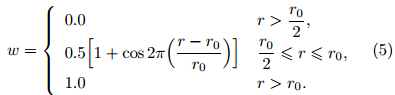
 , r isthe radius from the TC center and θ is the azimuth, and r0 is the radius out of which the TC componentbecomes zero, which is set to be 600 km here(theoreticallyit should be adjusted according to the size ofthe targeted TC vortex). The weighting function E(r)smoothly changes with radius from 0 at r = 0 to 1 atr = r0. In E(r), l is a parameter controlling the filtershape and is set to be 1/5 of r0 as in Kurihara et al.(1993).
The asymmetric part of the TC component isknown to play an important role in controlling TCmotion(Holland , 1983; Kurihara et al., 1993, 1995).We simply assume that the asymmetric part is reasonablyresolved in the analysis field although the axisymmetricflow in the inner core region is substantiallyweak compared to the actual TC. Therefore, inthe DI scheme, the TC vortex field is further decomposedinto the axisymmetric
The cycle run is the key of the DI scheme. Itspins up the axisymmetric TC vortex component asdone recently in Cha and Wang(2013). Each cyclerun is initialized at the initial model simulation timet0 and is integrated for 3 h. In the first cycle run, the axisymmetric TC vortex in the analysis field isrelocated to the observed TC center if the center ofthe vortex in the analysis field is deviated from thatobserved. In all the subsequent cycle runs, the axisymmetricTC vortex from the current cycle run isused to replace the axisymmetric vortex in the previouscycle run at t0. The cycle run is repeated until theintensity of the TC vortex from the last cycle run iscomparable to the observed TC intensity. To ensure asmooth merging of the axisymmetric TC vortex fromthe cycle run and the rest of the field at t0, we defineFt=0ax and Ft=3ax as the axisymmetric TC vortex both atthe initial time t0 and after a cycle run, and constructa new axisymmetric TC vortex by
The SN technique has been widely used in regionalclimate modeling(e.g., Kida et al., 1991; von Storch et al., 2000; Riette and Caya, 2002; Miguez-Macho et al., 2005; Cha et al., 2011). It allowsthe model to nudge only the selected component ina model simulation. For example, in most applications, the large-scale component or the driving fieldin a limited-area model is expected to remain closeto the observation. Such a large-scale nudging can bemathematically expressed as
The SN is a new option for the upper-air nudgingsince the ARW-WRF version 3.1. Currently the SNcan be applied to zonal and meridional wind components, potential temperature, and water vapor mixingratio in the ARW-WRF model. In a recent study, Cha and Wang(2013)used the large-scale SN in theoutmost model domain in their DI scheme to reduceerrors in the large-scale motion during the cycle runs.They nudged both the large-scale wind and temperaturefields in the mid-upper troposphere. In our application, the SN is applied only to the mid-upper troposphericwind field in the outermost domain. Notethat since our interest is to achieve realistic simulation, not prediction, of the TC motion, structure and intensity changes, we use the SN to preserve the largescalewind field with wavelengths longer than 1000 kmnot only during the cycle runs in the DI scheme butalso throughout the model simulation as discussed inthe following two sections.3. Typhoon Megi(2010), model settings, and experimental design3.1 An overview of Typhoon Megi(2010)
Typhoon Megi(2010) was the most powerful and longest lived TC over the western North Pacific(WNP) and South China Sea(SCS)in 2010. It wasfirst identified as a tropical disturbance by the JointTyphoon Warning Center(JTWC)on 12 October.The Japan Meteorological Agency(JMA) and JTWCbegan to monitor the low-level cyclonic circulation asa tropical depression(TD). The TD further intensifiedinto a tropical storm(TS), named Megi by JMAat 1200 UTC 12 October. Later, on 14 October, aneye of the storm could be clearly seen from satellite images, and thus JMA upgraded Megi to a severe tropicalstorm(STS) and JTWC upgraded it to a category-1typhoon. JMA upgraded Megi to a typhoon on 15 October.
As shown in Fig. 2, Megi initially moved northwestward and then turned west-southwestward. It experienceda rapid intensification from 16 to 18 Octoberduring which Megi attained its peak intensitywith the central sea level pressure(SLP)of 905 hPa and the maximum 10-m wind speed of 80 m s−1, theonly super typhoon over theWNP in 2010. Megi madel and fall over the Luzon Isl and in northern Philippinesat around 0325 UTC 18 October. It weakened toa category-2 typhoon immediately after its l and fallover the Luzon Isl and . After crossing the Luzon Isl and , Megi entered the SCS and turned northwestward and then suddenly northward. During its northwardturning over the SCS, Megi slowed down whilere-intensified from category-2 to category-4 with thecentral SLP of 935 hPa and the maximum 10-m sustainedwind speed of 57 m s−1. Early on 20 October, Megi turned north-northeastward. It then weakenedto a TS, and finally a TD, and made its second l and fallat Zhangpu in Fujian Province, China on 23 October and dissipated on the next day.
In addition to the distinct track and intensitychanges(Fig. 2), Megi also experienced remarkablestructure changes. For example, the storm size increasedrapidly during its rapid intensification stage.Its original eyewall experienced a breakdown when itcrossed the Luzon Isl and and redeveloped shortly afterit entered the SCS. A new outer eyewall formedat a larger radius as a result of the axisymmetrizationof outer spiral rainb and s(Fig. 3). In the meantime, a new inner eyewall re-formed in the eye region ofthe large outer eyewall, a double eyewall phenomenonnever being documented before.
The numerical simulations of Typhoon Megi presentedin this study were performed using the ARWWRFmodel version 3.3.1. The model atmosphereis fully compressible and nonhydrostatic. The modeluses the terrain-following, hydrostatic-pressure(σ)asthe vertical coordinate. The model domain is two-wayinteractive, triply nested. The three meshes have sizesof 455×375, 436×436, and 328×328 grid points withhorizontal grid spacings of 18, 6, and 2 km, respectively.The resolutions of the terrain height and l and use data for these meshes are 5 min, 2 min, and 30 s(about 9, 4, and 1 km), respectively. There are 36 unevenσ-levels for all meshes extending from the surfaceto the model top at 50 hPa. Both the 6- and 2-kmmeshes automatically move following the TC centerduring the simulation to allow the TC inner core tobe covered in the nested meshes(Fig. 4). The outermost18-km mesh is fixed during the model integration.Most of the results discussed below are the outputfrom the innermost mesh. The model physics include(1)the single-moment 6-class cloud microphysicsscheme(WSM6, Hong and Lim, 2006)for grid-scalemoist processes;(2)the Mellor-Yamada Nakanishi and Niino level-2.5 turbulence closure scheme(Nakanishi and Niino, 2004)for subgrid-scale vertical mixing withthe Monin-Obukhov similarity theory for surface fluxcalculations over the ocean where the roughness lengthfor momentum is modified for TC strength winds(Moon et al., 2007);(3)the Rapid Radiative TransferModel(RRTM)(Mlawer et al., 1997)for longwave radiationcalculation and Dudhia scheme(Dudhia, 1989)for shortwave radiation calculation;(4)the NOAHl and surface scheme(Ek et al., 2003)for l and surfaceprocesses; and (5)the Kain-Fritsch cumulus parameterizationscheme(Kain and Fritsch, 1990, 1993; Kain, 2004)for deep and shallow convection in the outermostdomain. We assume that convection can be roughlyresolved in the two inner nested meshes. Dissipativeheating is considered in all model meshes.
The model initial and lateral boundary conditionsfor both cycle runs and model simulations are interpolatedfrom the National Centers for Environment Prediction(NCEP)global final(FNL)analysis which hasa horizontal resolution of 1°×1° on 27 uneven pressurelevels. The daily sea surface temperature(SST)dataset at a 1°×1° resolution is also from the FNL. Thedetails for the DI and the experimental design for Typhoon Megi(2010) are discussed below.3.3 DI for Typhoon Megi
The DI scheme described in Section 2 was usedto initialize Typhoon Megi at 0000 UTC 15 October2010, which is about one day before the onset of rapidintensification(RI)of the storm. In the Megi case, after5 cycle runs, the model TC obtained the intensitycomparable to that observed in the JTWC best trackdata and achieved the structure typical of a strong TC.Figure 5 shows the SLP fields from the initial FNLanalysis and those from the first, third, and fifth cycleruns, respectively. In the initial FNL analysis field, the central SLP of the TC vortex is too weak comparedto that from the JTWC best track data(1002.1versus 956 hPa), mainly because the storm core wasnot resolved well by the coarse resolution FNL analysis.The vortex deepened gradually after each cyclerun and the TC vortex developed a compact inner corestructure, consistent with observations(Fig. 3). After5 cycle runs, the TC vortex reached an intensitywith a central SLP of 956.4 hPa and the maximum10-m sustained wind speed of 45.2 m s−1, comparedwell with the observed 956 hPa and 45 m s−1 in theJTWC best track data.
In addition to the storm intensity, the DI also producedthe realistic storm structure. As we can see fromthe azimuthal mean tangential wind given in Fig. 6, the axisymmetric structure of the TC vortex in theFNL analysis is quite weak and has the radius of maximumwind(RMW)of 140 km in the lower troposphere(Fig. 6a). After 1 cycle run, the storm started to intensify and contracted in its inner core size(Fig. 6b).After 3 cycle runs, the storm continued intensifyingwith the RMW reduced to about 60 km with a deepcyclonic circulation(Fig. 6c). After 5 cycle runs, thestorm further intensified and developed the structuretypical of a mature TC with the RMW of about 50km(Fig. 6d). Consistent with the primary circulation, the secondary circulation was also well developedthrough the cycle runs. As seen in Fig. 7, both the radialinflow in the boundary layer and the outflow in theupper troposphere are quite weak in the FNL analysis(Fig. 7a). After 3 and 5 cycle runs, both developedwell(Figs. 7c and 7d), showing typical axisymmetricstructure of a strong TC.
Since the DI scheme only spins up the axisymmetriccomponent of the TC vortex, it is also our interestto look at the asymmetric structure of the storm. Figure 8 shows the zonal-vertical cross-sections of totalwind speed and potential temperature across the TCcenter from the FNL analysis and from the DI after1, 3, and 5 cycle runs, respectively. We can see thatthe TC vortex in the FNL analysis shows an east-westasymmetry in total wind speed with stronger winds tothe east of the storm center(Fig. 8a). This asymmetryis maintained throughout the cycle runs(Figs.8b–d). The above results indicate that the DI substantiallyimproved the TC intensity and structure fromthe coarse-resolution FNL analysis.
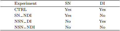
Four experiments were designed(Table 1)todemonstrate how the combined use of the DI scheme and the large-scale SN improves the subsequent simulationof Typhoon Megi. In the control(CTRL)experiment, both the DI scheme and the large-scale SNdescribed in Sections 2 and 3.3 were used throughoutthe simulation. In the second experiment(SN−NDI), the DI scheme was not used while the large-scale SNwas used throughout the simulation. In the third experiment(NSN−DI), the DI scheme was used while thelarge-scale SN was skipped in the simulation. In thelast experiment(NSN−NDI), neither the DI schemenor the large-scale SN was used in the simulation. Thelatter three simulations were designed as sensitivityexperiments to demonstrate the advantages of the DIscheme and the large-scale SN in realistic simulation of a real TC.
In all experiments, the initial time was 0000 UTC15 October 2010. As in the DI scheme, the initial and lateral boundary conditions and SST were interpolatedfrom the FNL analysis data with a 1°×1° resolution.The model was integrated for 168 h up to 0000 UTC22 October for each experiment. Therefore, the simulationcovered the initial RI period of Megi, the weakeningduring its l and fall over the Luzon Isl and , and itsre-intensification and sudden northward turning motion after it reentered the ocean over the SCS. In thenext section, we will demonstrate that the use of theDI scheme and the large-scale SN considerably improvesthe simulated storm track, structure, and intensitychanges.4. Results4.1 Storm track and intensity
Figure 9a shows the tracks of Typhoon Megi simulatedin the four experiments listed in Table 1 togetherwith the track from the JTWC best track data. Allexperiments simulated the west-northwestward movementin the first two days and the west-southwestwardmovement until the storm crossed the Luzon Isl and .The considerable difference among the four experimentsoccurred about one day after the storm crossedthe Luzon Isl and and reentered the ocean over theSCS. In particular, the difference is large between simulationswith and without the use of the large-scaleSN. The tracks from the experiments with the SN(SN−DI and SN−NDI)are in good agreement with theJTWC best track data, especially from CTRL with theDI. The improved track forecast in these two experimentscan be attributed to the improved large-scalecirculation in the simulations as a result of the use ofthe large-scale SN(see Section 4.3 below). The trackwith the DI is closer to the best track than that without the DI, suggesting that the better representationof the initial TC structure from the DI also contributesto the improved track simulation. The track errors inthe two experiments without the use of the SN are relativelylarge(Fig. 10a). The extremely large track errorsare related to the substantially delayed northwardturning after the storm entered the SCS, in particularfor the simulation without the DI(Fig. 10a). Only theCTRL experiment with both the DI and large-scaleSN captured the timing and location of the observednorthward turning motion over the SCS realistically(Fig. 9).
The simulated storm intensity also shows sensitivityto both the DI and the SN(right panels in Fig. 9).Overall, all experiments simulated well the intensitychange in terms of the central SLP and the maximumsustained surface wind speed. Namely, all experimentssimulated the rapid intensification of the observedstorm before it made l and fall over the LuzonIsl and , the rapid weakening after l and fall across theLuzon Isl and , and the re-intensification of the stormafter it reentered the ocean over the SCS. Nevertheless, the simulations with the DI in general producedthe storm intensity in better agreement with the besttrack data than those without the DI(Fig. 10b). Inparticular, the simulations without the DI show largenegative intensity biases in the first 2–3 days due tothe weak intensity of the initial TC vortex in the FNLanalysis. However, all experiments failed to reproducethe slow weakening and thus overestimated the stormintensity after 0600 UTC 20 October when the stormmoved north-northeastward over the SCS. This waspartially due to the ignorance of the negative oceanfeedback because the daily mean SST was used in allsimulations. Note that although large differences occurredbetween the experiments with and without theDI, the intensity bias show similar tendencies(Fig. 10b), indicating that the difference in storm track didnot contribute significantly to the intensity bias in theMegi case. The large intensity bias around 0600 UTC18 October in both CTRL and SN−NDI is related toslightly earlier l and fall of the storm in the simulationsthan in the observation. Note also that the intensitybiases are relatively large compared to the track errorseven though the DI scheme was used, indicatingthat it is still a challenge to realistically simulate TCintensity by high-resolution numerical models.
The above results show that the simulated stormtrack can be largely improved with the use of the largescaleSN, while the simulated storm intensity can beimproved with the use of the DI scheme, at least forthe first 6–12 h. Overall, the CTRL simulation withboth the DI and the large-scale SN reproduced boththe track and intensity changes better than any of theother three experiments. This suggests that the approachdescribed in Section 2 can be used to achieveimproved simulations of the track and intensity of realTC cases if a good global analysis is available and usedto drive a high-resolution regional atmospheric model.4.2 Storm structure change
A detailed verification of the three-dimensionalstructure of the simulated storm is impossible sincethere are few observations available over the openocean. Here we roughly compare the cloud/precipitationstructure based on the cloud/precipitationfeatures from satellite observations, such as theMIMIC-IR(Morphed Integrated Microwave Imageryat CIMSS, with infrared)images as shown in Fig. 11.Since the brightness temperature is highly correlatedwith deep convection and heavy precipitation, it isqualitatively comparable to the model simulated radarreflectivity near the surface, which reflects surface precipitation.
At 2000 UTC 15 October, just before the RIstarted, the storm displayed considerable convectiveasymmetric structure in the eyewall, with enhanced and wide convective area in the northeast quadrant and a much narrower eyewall to the south(Fig. 11a).An inner and an outer spiral rainb and s extended outwardfrom the eyewall to the southeast. The overallcloud/precipitation structure was simulated reasonablywell in the two experiments with the DI(CTRL and NSN−DI)though the simulation withoutthe SN(NSN−DI)produced convection too strong inthe southern eyewall(Figs. 12a and 12b). In sharpcontrast, the two experiments without the DI simulatedpartial eyewall structure with eyewall convectionto the south almost missing(Figs. 12c and 12d). Sincethe results shown in Figs. 11a–d are only after 20 hof model integration, it is suggested that the DI ofthe initial TC vortex significantly improved the stormstructure in the early model simulation.
By 2300 UTC 17 October, at the time just beforethe storm made l and fall over the Luzon Isl and , the storm developed double eyewall structure and increasedin its size with active outer spiral rainb and s tothe northeast and over the Luzon Isl and (Fig. 11b).The overall structure was simulated reasonably wellin all experiments except for the failure of the doubleeyewall structure at the given time in the simulation and the difference in the simulated storm position(Figs. 12e–h). Despite the failure in simulating thedouble eyewall structure just before the l and fall ofthe storm, all experiments simulated a double eyewallstructure after the storm made l and fall and movedover the Luzon Isl and as a result of the rapid contraction and then the weakening of the original eyewall and the sustaining of the strong outer quasi-symmetricrainb and s(figure omitted). Note that the differencebetween the experiments with and without the DI becomesinsignificant in Figs. 12e–h, suggesting that theDI affects the simulated storm structure mainly in thefirst day before the storm developed well in the Megicase.
Megi exhibited a drastic eyewall structure changeafter it crossed the Luzon Isl and and entered the SCS(Fig. 3). The original eyewall disappeared when thestorm moved over the Luzon Isl and . After the stormentered the SCS, it formed a new large eyewall as a resultof the axisymmetrization of the outer spiral rainb and .This is because the outer circulation/rainb and remained strong when the storm moved across the LuzonIsl and even though its inner core intensity substantiallyweakened(Figs. 3 and 11c). Similar featureshave been previously described for storms that crossedthe Luzon Isl and based on both observations and numericalsimulations(Wu et al., 2003, 2009; Chou et al., 2011). At the time given in Fig. 11c, the new eyewallwas at its formation stage with strong convectionto the northwest, a strong and wide convective spiralrainb and extending from the new eyewall to the southwest, and some loosely organized convective activitiesto the southeast. The overall structure, including theasymmetric structure, was simulated reasonably wellin all experiments(Figs. 12i–l). The phase of the convectiveasymmetries was better simulated in the twoexperiments with the DI(Figs. 12i and 12j). Thestorm simulated in NSN−NDI showed stronger eyewallconvection and was more axisymmetric than thestorm simulated in any other experiments(Fig. 12l).The storm in SN−NDI developed strong convection tothe northeast in the new eyewall(Fig. 12k)instead ofthe northwest in the observation(Fig. 11c).
Megi developed a double eyewall structure againas it re-intensified over the SCS(Fig. 11d). The developmentof the double eyewall structure was partly responsiblefor the observed weakening of the storm after0600 UTC 20 October. None of the experiments simulatedthe formation of the double eyewall structureas observed(Figs. 12m–p). Note that the CTL experimentproduced an apparent double eyewall structurebut not as typical as that observed(Fig. 12m). Asa result, all experiments failed to simulate the weakeningof Megi after 20 October. Nevertheless, overall, both the DI and the large-scale SN contributed to theimproved simulation of the storm structure evolutionalthough some discrepancies exist. The results fromCTRL could thus be analyzed to underst and the physicalmechanisms responsible for the structure changewhen Megi crossed the Luzon Isl and as well as the possibleterrain and l and mass effects of the Luzon Isl and in a future study.4.3 Effect of spectral nudging
We have already shown above that the large-scaleSN considerably improved the simulation of TyphoonMegi, in particular its track. This is due to the factthat the large-scale SN effectively preserved the largescaleenvironmental flow. This can be measured by theroot mean square error(RMSE)for any given variableof the large-scale component in the model simulationfrom the FNL analysis(namely, the driving field). Figure 13 shows the time series of the RMSEs for bothzonal and meridional winds at 500 hPa in the fourexperiments listed in Table 1. The RMSEs for theexperiments with and without the DI are quite closeto each other, indicating that the DI of the TC vortexhas little effect on the large-scale environmentalfield. In sharp contrast, the large difference occursbetween the experiments with and without the use ofthe large-scale SN. For example, throughout the 7-daysimulation, the RMSEs for both zonal and meridionalwinds are generally less than 0.6–0.7 m s−1 in the twoexperiments with the SN while they increased withtime almost linearly in the first 2–3 days and then remainedas large as about 2.2–2.5 m s−1, nearly 3–3.5times larger than those with the large-scale SN. Notethat the track errors remained small in the first 5-daysimulation even without the use of the large-scale SN(Fig. 10a). This is mainly because errors in the largescalewind field appeared in the midlatitude where theerror grows much faster than that in the tropics whilethe storm was located in the deep tropics. Nevertheless, the large errors in the large-scale wind field eventuallyled to large errors in the simulated storm trackin the last two days(Fig. 10a). The results thereforedemonstrate that the use of the large-scale SNeffectively preserves the environmental flow and thusimproves the simulation of storm motion.
Figure 14 shows the large-scale component ofgeopotential height at 500 hPa after 3-, 5-, and 7-day simulation in CTRL and NSN−DI experiments, respectively. The simulated large-scale geopotentialheight field in the experiment with the large-scale SN(CTRL simulation)shows little deviation from thatin the FNL analysis throughout the simulation(Figs.14a, 14c, and 14e). In the experiment without thelarge-scale SN(NSN−DI), the simulated large-scalecomponent of geopotential height field shows considerabledeviation from the FNL analysis(Figs. 14b, 14d, and 14f). The deviation increased with time in thesimulation without the SN. After the storm crossedthe Luzon Isl and , the WNP subtropical high weakened and retreated eastward in the FNL analysis(Fig. 14). The southerly wind west of the subtropical highsteered the storm northward around 20 October(Fig. 9). This was well simulated in the CTRL experimentwith the SN. In the experiment without the SN, thesimulated subtropical high is stronger than the observed, which led to a slightly faster movement and considerably delayed the northward turning of the simulatedstorm(Fig. 9). By the end of the 7-day simulation, considerable deviation in the large-scale geopotentialheight field is obvious. It is featured with thestrengthening of a ridge northeast of the simulatedstorm, leading to a westward track error in the experiments without the large-scale SN.
The results above demonstrated that the use ofthe SN reduced the model bias in the large-scale environmentalflow and thus improved the simulated stormtrack. Without the SN, the model bias in the simulatedlarge-scale environmental flow increased withtime and led to considerable bias in the simulatedstorm track. As a result, if the focus of a study isnot on how the TC affects the large-scale environmentalflow, the large-scale SN is an attractive approachto achieving the realistic simulations of a real TC in ahigh-resolution regional atmospheric model if a goodglobal analysis is available and used to drive the regionalmodel.5. Conclusions
In this study, we have presented a new approach, which combines a DI scheme with 3-h cycle runs and the large-scale SN, to achieving improved simulationsof a real TC, including its track, structure, and intensitychanges, using the advanced WRF model. TheDI scheme effectively provides realistic high-resolutioninitial conditions for the targeted TC. In this DIscheme, the axisymmetric component of the TC vortexin the coarse-resolution global analysis is replacedby the more realistic and dynamically-constrained axisymmetricTC vortex after each 3-h cycle run. Theasymmetric component is implicitly assumed to beresolved well in the global analysis field and is thuskept unchanged at the initial time of the cycle runs.The cycle run is terminated once the intensity of themodel TC is comparable to that observed. The DIscheme has been shown to be able to improve not onlythe simulated TC intensity but also the simulatedTC structure. To reduce the bias in the simulatedlarge-scale environmental flow, which controls the TCmotion, the large-scale SN approach is used to thewind field in the outermost model domain. The SNis applied not only during the cycle runs but alsothroughout the subsequent model simulation.
The effectiveness of the proposed approach hasbeen demonstrated with a case study of Typhoon Megi(2010) using the ARW-WRF model. The controlexperiment with the proposed approach realisticallyreproduced many aspects of Typhoon Megi in aweek-long simulation. The model simulated quite wellthe storm track, and structure and intensity changes.In particular, the model captured not only the rapidintensification and the size increase before Megi madel and fall over the Luzon Isl and , but also its drasticstructure changes when Megi crossed the Luzon Isl and in the northern Philippines. The control simulationalso reproduced the re-intensification and the formationof the new large eyewall after Megi entered theSCS. The results from several sensitivity experimentsshow that the use of the large-scale SN contributedgreatly to the improved track simulation, in particularfor the simulation after three days, while the use ofthe DI scheme mainly improved the storm intensity and structure in the first 2–3-day simulation. Overall, the results demonstrate that the combined use of theDI and the SN is quite effective and ideal for achievingimproved simulation for the process studies focusingon TC inner-core dynamics, and structure and intensitychanges. Our detailed studies to underst and therapid intensification, size change, and intensity and structure changes in Typhoon Megi are underway and the results will be reported separately.
Because the main purpose of this paper is to introducethe new approach, its effectiveness has beenexamined by one simulation. However, results fromsome extra experiments with different initial times arealso promising(figure omitted). Nevertheless, morecase studies are required to demonstrate the robustness and applicability of the proposed approach infuture studies. In addition, the DI scheme can becombined with a four-dimensional data assimilationsystem during the cycle runs to further improve theinitial TC structure. Note that although the approachhas been developed based on the ARW-WRF model, itcan be easily transferred to any other high-resolutionmodels since it was constructed as an individual module.
Finally, it should be mentioned that the approachproposed in this study has some limitations. Firstly, the approach is better applied to well-defined TC systemssince if the system is too weak, the axisymmetriccomponent may not be well determined. Secondly, the cycle runs only spin up the axisymmetric componentof a TC. As a result, if a storm has significantasymmetric structure in particular in the inner coreregion, the approach will not work properly. Thirdly, since the azimuthal mean is performed to constructthe axisymmetric TC vortex after each cycle run, oncethe TC is approaching any topography, the approachwill have errors since extrapolations need to be used.As a result, when the targeted TC is too close to topography, the approach is not recommended. In thatcase, the earlier initial time can be considered for thesimulation. This may not be a barrier for the applicationof the proposed approach since it is proposed toimprove numerical simulations not prediction. Nevertheless, it will be a good topic for a future studyto extend the current work to include the asymmetricstructure, which is beyond the scope of this work.
Acknowledgments. The authors are gratefulto two anonymous reviewers for their helpful comments.
 and asymmetric(Fas = Fhv − Fax)components. In thecycle runs described below, only the axisymmetric TCcomponent is spun up while the basic field, the asymmetricTC component, and the non-TC perturbationfield remain unchanged.2.2 Cycle runs and vortex construction

Fig. 2.(a)Track of Typhoon Megi(2010) at 6-h intervals, and the time series of(b)central sea level pressure(hPa) and (c)maximum sustained 10-m wind speed(m s−1)of the JTWC best track data from 0000 UTC 12 to 0000 UTC 24October 2010. 
Fig. 3. Satellite images at given times during 15–21 October 2010, showing the inner core size increase before Typhoon Megi(2010) made l and fall over the Luzon Isl and and the remarkable structure changes when the typhoon crossed theLuzon Isl and . Courtesy of the US Naval Research Lab. 
Fig. 4. The triply-nested, movable mesh model domainsused for Typhoon Megi simulation in this study. 
Fig. 5. The sea level pressure field(hPa; shaded)superimposed with the surface winds(wind bars)from(a)the NCEPFNL analysis; and from the dynamical initialization after(b)1 cycle run, (c)3 cycle runs, and (d)5 cycle runs forTyphoon Megi at 0000 UTC 15 October 2010. 
Fig. 6. Radial-vertical structure of the azimuthal mean tangential wind from(a)the NCEP FNL analysis and from thedynamical initialization after(b)1 cycle run, (c)3 cycle runs, and (d)5 cycle runs for Typhoon Megi at 0000 UTC 15October 2010. 
Fig. 7. As in Fig. 6, but for the azimuthal mean radial wind. 
Fig. 8. Zonal-vertical cross-sections of the total horizontal wind speed(m s−1; shaded) and potential temperature(K;contour)across the TC center from the FNL analysis(a) and from the DI after(b)1 cycle run, (c)3 cycle runs, and (d)5 cycle runs valid at 0000 UTC 15 October 2010. 
Fig. 9.(a)Track of Typhoon Megi, and the time series of(b)central sea level pressure(hPa) and (c)maximumsustained 10-m wind speed(m s−1)from 0000 UTC 15 to 0000 UTC 22 October 2010 from the JTWC best track data(black) and from the four experiments listed in Table 1. 
Fig. 10. Simulated TC(a)track errors(km) and (b)intensity biases(m s−1)in the four experiments listed in Table 1. 
Fig. 11. The MIMIC-IR images at(a)2000 UTC 15, (b)2300 UTC 17, (c)0100 UTC 19, and (d)0900 UTC 20October. The labels at top left of each panel denote the NHC(National Hurricane Center)-reported maximum sustainedwinds, and those at top right of each panel denote the temporal separation from the microwave overpass nearest in time. 
Fig. 12. The model simulated radar reflectivity at σ = 0.9215 at(a–d)2000 UTC 15, (e–h)2300 UTC 17, (i–l)0100UTC 19, and (m–p)0900 UTC 20 October 2010 from experiments(a, e, i, m)CTRL, (b, f, j, n)NSN−DI, (c, g, k, o)SN−NDI, and (d, h, l, p)NSN−NDI. 
Fig. 13. Time evolution the RMSEs of the large-scale(a)zonal and (b)meridional winds at 500 hPa in the fourexperiments listed in Table 1. 
Fig. 14. Filtered geopotential height fields at 500 hPa at 0000 UTC(a, b)18, (c, d)20, and (e, f)22 October 2010from the FNL in black and from the(a, c, e)control experiment and (b, d, f)NSN−DI in red.

| [1] | Bender, M. A., I. Ginis, and Y. Kurihara, 1993: Numerical simulations of tropical cyclone-ocean interaction with a high-resolution coupled model. J. Geophys. Res., 98(D12), 23245-23263. |
| [2] | Braun, S. A., 2002: A cloud-resolving simulation of Hurricane Bob (1991): Storm structure and eyewall buoyancy. Mon. Wea. Rev., 130(6), 1573-1592. |
| [3] | ——, 2006: High-resolution simulation of Hurricane Bonnie (1998). Part II: Water budget. J. Atmos. Sci., 63(1), 43-64. |
| [4] | ——, and W. K. Tao, 2000: Sensitivity of high-resolution simulations of Hurricane Bob (1991) to planetary boundary layer parameterizations. Mon. Wea. Rev., 128(12), 3941-3961. |
| [5] | ——, M. T. Montgomery, and Z. -X. Pu, 2006: High-resolution simulation of Hurricane Bonnie (1998). Part I: The organization of eyewall vertical motion. J. Atmos. Sci., 63(1), 19-42. |
| [6] | Cha, D.- H., C. -S. Jin, D. -K. Lee, et al., 2011: Impact of intermittent spectral nudging on regional climate simulation using Weather Research and Forecasting model. J. Geophys. Res., 116, D10103, doi: 10.1029/2010JD015069. |
| [7] | ——, and Y. Q. Wang, 2013: A dynamical initialization scheme for real-time forecasts of tropical cyclones using the WRF model. Mon. Wea. Rev., 141(3), 964-986. |
| [8] | Chou K.- H., C.- C. Wu, Y. Wang, and C.- H. Chih, 2011: Eyewall evolution of typhoons crossing the Philippines and Taiwan: An observational study. Terr. Atmos. Ocean. Sci., 22(6), 535-548. |
| [9] | Cram, T. A., J. Persing, M. T. Montgomery, et al., 2007: A Lagrangian trajectory view on transport and mixing processes between the eye, eyewall, and environment using a high-resolution simulation of Hurricane Bonnie (1998). J. Atmos. Sci., 64(6), 1835-1856. |
| [10] | Davis, C. A., and L. F. Bosart, 2001: Numerical simulations of the genesis of Hurricane Diana (1984). Part I: Control simulation. Mon. Wea. Rev., 129(8), 1859-1881. |
| [11] | ——, and S. Low-Nam, 2001: The NCAR-AFWA Tropical Cyclone Bogussing Scheme. Air Force Weather Agency (AFWA) Rep., 12 pp. [Available online at http://www.mmm.ucar.edu/mm5/mm5v3/tc-bogus.html.] |
| [12] | ——, and L. F. Bosart, 2002: Numerical simulations of the genesis of Hurricane Diana (1984). Part II: Sensitivity of track and intensity prediction. Mon. Wea. Rev., 130(5), 1100-1124. |
| [13] | ——, W. Wang, S. S. Chen, et al., 2008: Prediction of landfalling hurricanes with the advanced hurricane WRF model. Mon. Wea. Rev., 136(6), 1990-2005. |
| [14] | Dudhia, J., 1989: Numerical study of convection observed during the Winter Monsoon Experiment using a mesoscale two-dimensional model. J. Atmos. Sci., 46(20), 3077-3107. |
| [15] | Ek, M. B., K. E. Mitchell, Y. Lin, et al., 2003: Implementation of Noah land surface model advances in the National Centers for Environmental Prediction operational mesoscale Eta model. J. Geophys. Res., 108, 8851, doi:10.1029/2002JD003296. |
| [16] | Feser, F., and H. von Storch, 2008: A dynamical downscaling case study for typhoons in Southeast Asia using a regional climate model. Mon. Wea. Rev., 136(5), 1806-1815. |
| [17] | Goerss, J. S., and R. A. Jeffries, 1994: Assimilation of synthetic tropical cyclone observations into the Navy Operational Global Atmospheric Prediction System. Wea. Forecasting, 9(4), 557-576. |
| [18] | Hendricks, E. A., M. S. Peng, X. -Y. Ge, et al., 2011: Performance of a dynamic initialization scheme in the Coupled Ocean-Atmosphere Mesoscale Prediction System for Tropical Cyclones (COAMPS-TC). Wea. Forecasting, 26(5), 650-663. |
| [19] | Hogsett, W., and D. -L. Zhang, 2009: Numerical simulation of Hurricane Bonnie (1998). Part III: Energetics. J. Atmos. Sci., 66(9), 2678-2696. |
| [20] | ——, and ——, 2010: Genesis of Typhoon Chanchu (2006) from a westerly wind burst associated with the MJO. Part I: Evolution of a vertically tilted precursor vortex. J. Atmos. Sci., 67(12), 3774-3792. |
| [21] | ——, and ——, 2011: Genesis of Typhoon Chanchu (2006) from a westerly wind burst associated with the MJO. Part II: Roles of deep convection in tropical transition. J. Atmos. Sci., 68(6), 1377-1396. |
| [22] | Holland, G. J., 1983: Tropical cyclone motion: Environmental interaction plus a beta effect. J. Atmos. Sci., 40(2), 328-342. |
| [23] | Hong, S. -Y., and J. -O. J. Lim, 2006: The WRF single-moment 6-class microphysics scheme (WSM6). J. Korean Meteor. Soc., 42(2), 129-151. |
| [24] | Kain, J. S., 2004: The Kain-Fritsch convective parameterization: An update. J. Appl. Meteor., 43(1), 170-181. |
| [25] | ——, and J. M. Fritsch, 1990: A one-dimensional entraining/detraining plume model and its application in convective parameterization. J. Atmos. Sci., 47(23), 2784-2802. |
| [26] | ——, and J. M. Fritsch, 1993: Convective parameterization for mesoscale models: The Kain-Fritsch scheme. The Representation of Cumulus Convection in Numerical Models, Meteor. Monogr., Amer. Meteor. Soc., 24, 165-170. |
| [27] | Kida, H., T. Koide, H. Sasaki, et al., 1991: A new approach for coupling a limited area model to a GCM for regional climate simulations. J. Meteor. Soc. Japan, 69, 723-728. |
| [28] | Kurihara, Y., M. A. Bender, and R. J. Ross, 1993: An initialization scheme of hurricane models by vortex specification. Mon. Wea. Rev., 121(7), 2030-2045. |
| [29] | ——, ——, R. E. Tuleya, et al., 1995: Improvements in the GFDL Hurricane Prediction System. Mon. Wea. Rev., 123(9), 2791-2801. |
| [30] | Kwon, I. -H., and H. -B. Cheong, 2010: Tropical cyclone initialization with a spherical high-order filter and an idealized three-dimensional bogus vortex. Mon. Wea. Rev., 138(4), 1344-1367. |
| [31] | Leslie, L. M., and G. J. Holland, 1995: On the bogussing of tropical cyclones in numerical models: A comparison of vortex profiles. Meteor. Atmos. Phys., 56(1-2), 101-110. |
| [32] | Li, X. -L., and Z.- X. Pu, 2008: Sensitivity of numerical simulation of early rapid intensification of Hurricane Emily (2005) to cloud microphysical and planetary boundary layer parameterizations. Mon. Wea. Rev., 136(12), 4819-4838. |
| [33] | Liu, B., and L. Xie, 2012: A scale-selective data assimilation approach to improving tropical cyclone track and intensity forecasts in a limited-area model: A case study of Hurricane Felix (2007). Wea. Forecasting, 27(1), 124-140. |
| [34] | Liu, Y. B., D. -L. Zhang, and M. K. Yau, 1997: A multiscale numerical study of Hurricane Andrew (1992). Part I: Explicit simulation and verification. Mon. Wea. Rev., 125(12), 3073-3093. |
| [35] | ——, ——, and ——, 1999: A multiscale numerical study of Hurricane Andrew (1992). Part II: Kinematics and inner-core structures. Mon. Wea. Rev., 127(11), 2597-2616. |
| [36] | Ma, S. -H., A. -X Qu, and Y. Wang, 2007: The performance of the new tropical cyclone track prediction system of the China National Meteorological Center. Meteor. Atmos. Phys., 97(1-4), 29-39. |
| [37] | Miguez-Macho, G., G. L. Stenchikov, and A. Robock, 2005: Regional climate simulations over North America: Interaction of local processes with improved large-scale flow. J. Climate, 18(8), 1227-1246. |
| [38] | Mlawer, E. J., S. J. Taubman, P. D. Brown, et al., 1997: Radiative transfer for inhomogeneous atmospheres: RRTM, a validated correlated-k model for the longwave. J. Geophys. Res., 102(D14), 16663-16682. |
| [39] | Moon, I.- J., I. Ginis, T. Hara, et al., 2007: A physics-based parameterization of air-sea momentum flux at high wind speeds and its impact on hurricane intensity predictions. Mon. Wea. Rev., 135(8), 2869-2878. |
| [40] | Musgrave, K. D., C. A. Davis, and M. T. Montgomery, 2008: Numerical simulations of the formation of Hurricane Gabrielle (2001). Mon. Wea. Rev., 136(8), 3151-3167. |
| [41] | Nakanishi, M., and H. Niino, 2004: An improved Mellor-Yamada Level-3 model with condensation physics: Its design and verification. Boundary-Layer Meteor., 112(1), 1-31. |
| [42] | Peng, M. S., B.- F. Jeng, and C.- P. Chang, 1993: Forecast of typhoon motion in the vicinity of Taiwan during 1989-90 using a dynamical model. Wea. Forecasting, 8(3), 309-325. |
| [43] | Pu, Z. -X., and S. A. Braun, 2001: Evaluation of bogus vortex techniques with four -dimensional variational data assimilation. Mon. Wea. Re., 129(8), 2023-2039. |
| [44] | Riette, S., and D. Caya, 2002: Sensitivity of short simulations to the various parameters in the new CRCM spectral nudging. Research Activities in Atmospheric and Oceanic Modelling, edited by H. Ritchie, WMO/TD - No 1105, Report No. 32, 7.39-7.40. |
| [45] | Rogers, R., 2010: Convective-scale structure and evolution during a high-resolution simulation of tropical cyclone rapid intensification. J. Atmos. Sci., 67(1), 44-70. |
| [46] | Rogers, , M. L. Black, S. S. Chen, et al., 2007: An evaluation of microphysics fields from mesoscale model simulations of tropical cyclones. Part I: Comparisons with observations. J. Atmos. Sci., 64(6), 1811-1834. |
| [47] | Tallapragada, V., Y. C. Kwon, Q. Liu, et al., 2012: Operational implementation of high-resolution triply-nested HWRF at NCEP/EMC - A major step towards addressing intensity forecast problem. The 30th Conference on Hurricanes and Tropical Meteorology, Amer. Meteor. Soc., 15-20 April 2012, Ponte Vedra Beach, Florida. |
| [48] | Ueno, M., 1989: Operational bogussing and numerical prediction of typhoon in JMA. JMA/NPD Tech. Rep., 28, 48 pp. |
| [49] | van Nguyen, H., and Y.- L. Chen, 2011: High-resolution initialization and simulations of Typhoon Morakot (2009). Mon. Wea. Rev., 139(5), 1463-1491. |
| [50] | von Storch, H., H. Langenberg, and F. Feser, 2000: A spectral nudging technique for dynamical downscaling purposes. Mon. Wea. Rev., 128(10), 3664-3673. |
| [51] | Wang, Y. Q., 1998: On the bogusing of tropical cyclones in numerical models: The influence of vertical structure. Meteor. Atmos. Phys., 65(3-4), 153-170. |
| [52] | ——, 2001: An explicit simulation of tropical cyclones with a triply nested movable mesh primitive equation model: TCM3. Part I: Model description and control experiment. Mon. Wea. Rev., 129(6), 1370-1394. |
| [53] | Wu, C.- C., K. -H. Chou, H. -J. Cheng, et al., 2003: Eyewall contraction, breakdown and reformation in a landfalling typhoon. Geophys. Res. Lett., 30(17), 1887, doi: 10.1029/2003GL017653. |
| [54] | ——, H. J. Cheng, Y. Q. Wang, et al., 2009: A numerical investigation of the eyewall evolution of a landfalling typhoon. Mon. Wea. Rev., 137(1), 21-40. |
| [55] | Yang, M. -J., D.- L. Zhang, and H. -L. Huang, 2008: A modeling study of Typhoon Nari (2001) at landfall. Part I: Topographic effects. J. Atmos. Sci., 65(10), 3095-3115. |
| [56] | ——, ——, X. -D. Tang, et al., 2011: A modeling study of Typhoon Nari (2001) at landfall. Part II: Structural changes and terrain-induced asymmetries. J. Geophys. Res., 116, D09112, doi: 10.1029/2010JD015445. |
| [57] | Yau, M. K., Y. B. Liu, D. -L. Zhang, et al., 2004: A multiscale numerical study of Hurricane Andrew (1992). Part VI: Small-scale inner-core structures and wind streaks. Mon. Wea. Rev., 132(6), 1410-1433. |
| [58] | Zhang, D. -L., Y. B. Liu, and M. K. Yau, 2000: A multiscale numerical study of Hurricane Andrew (1992). Part III: Dynamically-induced vertical motion. Mon. Wea. Rev., 128(11), 3772-3788. |
| [59] | ——, ——, and ——, 2001: A multiscale numerical study of Hurricane Andrew (1992). Part IV: Unbalanced flows. Mon. Wea. Rev., 129(1), 92-107. |
| [60] | ——, ——, and ——, 2002: A multiscale numerical study of Hurricane Andrew ( 1992). Part V: Inner-core thermodynamics. Mon. Wea. Rev., 130(11), 2745-2763. |
| [61] | ——, L. Tian, and M. J. Yang, 2011: Genesis of Typhoon Nari (2001) from a mesoscale convective system. J. Geophys. Res., 116, D23104, doi:10.1029/2011JD016640. |
| [62] | Zhang, Q.- H., S. -J. Chen, Y.- H. Kuo, et al., 2005: Numerical study of a typhoon with a large eye: Model simulation and verification. Mon. Wea. Rev., 133(4), 725-742. |
| [63] | Zhu, T., D. -L. Zhang, and F. Z. Weng, 2004: Numerical simulation of Hurricane Bonnie (1998). Part I: Eyewall evolution and intensity changes. Mon. Wea. Rev., 132(1), 225-241. |
| [64] | ——, and ——, 2006: Numerical simulation of Hurricane Bonnie (1998). Part II: Sensitivity to varying cloud microphysical processes. J. Atmos. Sci., 63(1), 109-126. |
| [65] | Zhang, X. Y., Q. N. Xiao, and P. J. Fitzpatrick, 2007: The impact of multisatellite data on the initialization and simulation of Hurricane Lili’s (2002) rapid weakening phase. Mon. Wea. Rev., 135(2), 526-548. |
| [66] | Zou, X. L., and Q. N. Xiao, 2000: Studies on the initialization and simulation of a mature hurricane using a variational bogus data assimilation scheme. J. Atmos. Sci., 57(6), 836-860. |