 2013, Vol. 27
The Chinese Meteorological Society
Article Information
- ZHANG Shuwen, LIU Yanhua and ZHANG Weidong. 2013.
- Ensemble Square Root Filter Assimilation of Near-Surface Soil Moisture and Reference-Level Observations into a Coupled Land Surface-Boundary Layer Model
- J. Meteor. Res., 27(4): 541-555
- http://dx.doi.org/10.1007/s13351-013-0402-6
-
Article History
- Received August 31, 2012
- in final form January 15, 2013


Modeling l and -atmosphere interaction has becomean important component of research in earthsystem sciences. The l and surface and atmosphericboundary layer compose a tightly coupled system withcomplicated interactions that modulate weather and climate variability(Boussetta et al., 2008; vanden Hurk et al., 2011; Yang and Shen, 2010). Soil moistureplays an important role in these interactions, largelycontrolling the partitioning of surface-atmosphere energytransfer into fluxes of sensible and latent heat.Realistic simulations of soil moisture are necessaryfor accurate forecasts using numerical weather prediction(NWP)models. An incorrect initialization of soilmoisture may lead to errors in the structure of theplanetary boundary layer(PBL) and possibly the developmentof precipitation, which in turn leads to furthererrors in soil moisture estimates. Soil moistureinitialization not only plays an important role in theprediction of precipitation but also affects the simulationof l and surface processes(Svensson et al., 2011;Koster et al., 2009; Li et al., 2007; Liu et al., 2010).
The representation of the PBL is an importantcomponent of any atmospheric model used for studiesof weather and climate, regardless of the scale ofinterest. A more accurate initialization of the PBLstructure has been shown to improve short-range forecastsof local thermally-driven flows in a mesoscalemodel and to positively influence forecasts of cyclogenesis, convective outbreaks, and frontal propagationin a large-scale NWP model(Hacker and Snyder, 2005). The accuracy of the initial PBL structure alsoinfluences three-dimensional background fields derivedfrom NWP models for use in process studies(such asstudies of air quality and plume dispersion)(Rémy and Bergot, 2009).
The initialization of NWP models is complicatedby a relative lack of observations of soil moisture and the state of the PBL. One alternative approach isto use data assimilation techniques within the modelframework to retrieve soil moisture profiles or the PBLstructure, thus combining direct or indirect observationswith model predictions. For example, remotesensing radiometric observations of surface temperaturecan be used to constrain surface soil moisture and heat fluxes(Reichle et al., 2010)through assimilatingmicrowave brightness temperature or satelliteretrieval of near-surface soil moisture into an off-linel and surface model(LSM)(Crow and van den Berg, 2010; Walker et al., 2001; Zhang et al., 2005, 2011).In addition to remote sensing measurements, st and ardground-based meteorological observations may be assimilatedinto a single column model(SCM)to estimatethe state of the l and surface(Hacker and Snyder, 2005; Hacker and Rostkier-Edelstein, 2007; Hess, 2001; Mahfouf, 1991). These ground-based observationsare rich, accurate, and often dense. Combinationsof different types of observations can also be usedto estimate soil moisture or PBL profiles. For example, Seuffert et al.(2003)assimilated both screenlevelparameters(e.g., 2-m temperature and specifichumidity) and satellite observations of 1.4 GHz brightnesstemperature to predict sensible heat fluxes, rootzones, and near-surface soil moisture. Similarly, Margulis and Entekhabi(2003)assimilated both radiometricsurface temperature and screen-level meteorologicalvariables(temperature and humidity)into a modelof the atmospheric boundary layer and l and surface toestimate surface heat fluxes and the states of the l and surface and PBL.
A number of different data assimilation approacheshave been adopted for use in constraining thestates of the l and surface and PBL, from simple directinsertion to complex flow-dependent ensemble-basedmethods. For example, optimal interpolation(OI)based on statistically derived soil-atmosphere characteristicshas been used to correct the soil moisture field(Mahfouf, 1991), while nudging and incremental updatemethods have been used to improve the initialPBL structure in a mesoscale model(Ruggiero et al., 1996). Other studies have used variational analysis toretrieve soil moisture as the minimum of a cost functionthat expresses the difference between observations and a specified background state(Seuffert et al., 2003;Zhang et al., 2007). Variational data assimilation techniqueshave also been used to retrieve soil moistureor PBL profiles(Reichle et al., 2001; Margulis and Entekhabi, 2003). Ensemble Kalman filters(EnKF) and other ensemble-based data assimilation methodshave also been widely used to constrain soil moisture and the structure of the PBL(Reichle and McLaughlin, 2002; Hacker and Rostkier-Edelsten, 2007; Tian et al., 2008; Zhang et al., 2010). These ensemblebasedmethods are able to capture the transient coupling and decoupling of the l and surface/PBL with thefree atmosphere aloft. Furthermore, they provide flowdependentestimates of background error covariance, including non-stationary and anisotropic correlationsbetween observations and model background states.This capability has proved very useful for skillful estimationof the PBL state.
Different data assimilation methods have beencompared to assess their relative skills for estimatingsoil moisture. Walker et al.(2001)compared directinsertion with the extended Kalman filter(EKF)method, finding that the latter is superior to the formerwith a quicker retrieval of the soil moisture profile.Reichle et al.(2002)showed that the EnKF methodprovided a slightly better estimate of soil moisturethan the EKF method. Zhou et al.(2006)comparedthe performance of EnKF for estimating soil moisturewith that of a sequential importance resampling particlefilter(which can give exact solutions for largeensemble sizes). They showed that EnKF providesa good approximation for non-normal, nonlinear l and surface problems despite its intrinsic assumption ofnormality.
The studies mentioned above have focused on estimatingsoil moisture profiles or PBL states separately.In this study, we estimate the soil moistureprofile and the PBL state simultaneously by assimilatingeither near surface soil moisture observationsalone or a suite of observations that includes nearsurface soil moisture, 2-m temperature and humidity, and 10-m horizontal wind. We also evaluate the contributionsof each observation to improving the estimatedsoil moisture profile, surface heat fluxes, and PBL state. The data assimilation is performed usingan unperturbed-observation ensemble square rootfilter(EnSRF)(Whitaker and Hamill, 2002), and the background forecasts are generated using a onedimensional(1D)coupled l and surface-boundary layermodel(CLS-BLM). The CLS-BLM contains the sameparameterizations as the Weather Research and Forecasting(WRF)model for sub-grid scale processes associatedwith the PBL, surface layer and l and surface(Hacker and Rostkier-Edelstein, 2007; Pagowski et al., 2005). Section 2 briefly introduces the CLS-BLM and the data assimilation algorithm. Section 3 describesthe experimental setup. Section 4 documents experimentalresults, including estimated soil moisture profiles, surface heat fluxes, PBL profiles, and sensitivityto observational errors. Section 5 provides a summary and discussion of the results.2. Model description and assimilation algorithm2.1 One-dimensional column model
This study uses the 1D column model CLS-BLM.CLS-BLM has the same physical parameterizations astheWRF model, and is forced externally by tendenciesderived from WRF forecasts(e.g., horizontal advection, downward short- and long-wave radiative fluxes and geostrophic wind). The PBL is simulated usingthe Mellor-Yamada-Janji´c scheme(Janjić et al., 2001) and l and surface processes are modeled using the NoahLSM(Chen and Dudhia, 2001).The Noah LSM, which was initially developed in1993, is directly related to many hydrologic models.
The model framework is based on a 1D approach tosoil-vegetation-atmosphere interactions that solves thecoupled energy and water budgets at the l and surface and within the unsaturated zone. Noah LSMis a st and -alone model; it can either be run off-line(driven by atmospheric forcings)or coupled with anatmospheric model. The model state variables includesoil moisture and soil temperature in 4 layers, skintemperature(bare soil or vegetation), canopy waterstorage, and a variety of storage variables related tosnow processes(Ek et al., 2003). The Noah LSM hasbeen extensively tested over a wide range of climateregimes. Recent improvements to the model have beendocumented by Niu et al.(2011) and Yang Zong-Lianget al.(2011).
The column model is adopted because it is easy touse in ensemble-based data assimilation experimentswhile maintaining the complexity of the original WRFmodel with respect to the PBL structure and l and atmosphereinteractions. The latter feature is essentialfor this study. Detailed descriptions of the CLS-BLMhave been provided by Pagowski et al.(2005) and Hacker and Rostkier-Edelstein(2007).2.2 Data assimilation algorithm
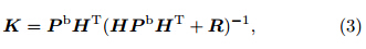
The ensemble-based data assimilation methodgenerally takes one of two forms: the stochastic filteror the deterministic filter. The latter approachis designed to avoid sampling errors associated withthe use of “perturbed observations” in the stochasticfilter. A variety of deterministic filters have beenproposed, including the ensemble transform Kalmanfilter, the ensemble adjustment Kalman filter, and En-SRF(Whitaker and Hamill, 2002). Here, we use En-SRF for convenience. Let xb be an m-dimensionalbackground vector, with x the sum of the ensemblemean x and x' the deviation from the ensemble mean(i.e., x = x + x'). Let y be a p-dimensional vectorof observations. In this study, y is composed ofobservations of soil moisture(θ°), 2-m temperature(T°), 2-m humidity(Q°), and 10-m horizontal wind(V°). The observation operator H transforms modelstates into the observational space. Pb is the m×mdimensionalbackground error covariance matrix, and R is the p × p-dimensional observational error covariancematrix. The minimum variance estimate of theerror in the analysis xa is formulated for EnSRF as
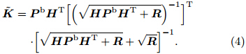
where K is the Kalman gain given by and

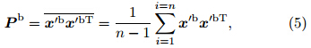
 is expressed asThe superscript T st and s for the matrix transpose. Pbis calculated according towhere n is the ensemble size.
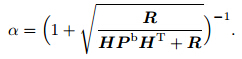
HPbHT and R reduce to scalars for an individualobservation. Assuming = αK(with a constantα), then a scalar quadratic equation for α can be obtainedwith the solution
An observing system simulation experiment(OSSE)is designed to reduce the interference of modelerrors. The true model states are assumed to be exactlyknown and the observations are generated byadding known r and om errors to the true model states.An OSSE is carried out between 13 and 29 August2003 at a single point with sparse, flat l and cover locatedat 37.6°N, 96.7°W. The weather during the testingperiod was fine, with no large advection processesor precipitation.
The initial PBL conditions and surface radiationare drawn from the WRF climatology, with thegeostrophic wind forcing set to 3 and –9 m s−1. Themodel is configured to run on 60 non-uniform verticallevels with the lowest model level at 45 m above groundlevel. T°, Q°, and V o are accordingly not predictedby the model; rather, they are calculated accordingto Monin-Obukhov similarity. The observation operatorH is not explicitly needed(Reichle et al., 2002).Forecasts were initiated at 0300 UTC with a horizontalspacing of 4 km and a time step of 60 s.
Rather than using the 4-layer discretization of thesoil column in the original Noah LSM, we divide the1-m soil column into 50 layers. The thickness of thetopmost layer is 1 cm, and the thickness of all remaininglayers is 2 cm. This approach increases the accuracyof the estimates and provides a fair comparisonwith previous data assimilation results using an offlineLSM. Additional details of the data assimilationenvironment are listed in Table 1.
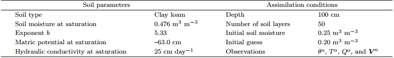
We adopt a relatively large ensemble of 80 memberswhen comparing the OSSE with model states.The initial ensemble of PBL state profiles is constructedby first r and omly selecting two forecasts fromWRF real-time forecasts at a 12-h lead time, then averaging them with weighting coefficients μ and 1–μ(with μ sampled from a uniform distribution U[0, 1]).The initial soil moisture is intentionally poor to accountfor the poor knowledge of actual soil moisture, with an initial value of 0.2 m3 m−3(approximatelyhalf the saturated soil moisture). The initial ensembleof soil moisture is generated by adding a normallydistributedr and om field with a mean of zero and ast and ard deviation(STD)of 0.05 m3 m−3 to the initialguess. Observational errors are represented by temporallyuncorrelated additive Gaussian noise with STDsof 1 K for T°, 0.8 g kg−1 for Q°, 1.4 m s−1 for |V°|, and 0.03 m3 m−3 for θ°. The assimilation time intervalranges from 24 to 0.5 h. Further details are providedin Section 4.
We use the mean absolute error(MAE)to quantitativelycompare estimates by different approaches.MAE is defined for an estimate f and its true value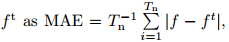 where Tn is the numberof the verification times. The benefit of the estimaterelative to an open loop simulation(i.e., an 80-member ensemble forecast without data assimilationwith the same ensemble members and initial conditionsas the assimilation system)is estimated usingthe relative MAE reduction(RMR)
RMR =(MAEOP − MAE)/MAEOP × 100%,
where MAEOP is the mean absolute error from theopen loop simulation.4. Results and analysis4.1 Results from assimilating only the nearsurface soil moisture observationsPrevious assimilation studies have used off-linemeteorological forcing data to drive the LSM withoutany coupling between the l and surface and the atmospherealoft. Here, averaged soil moisture estimatesare calculated in four representative layers with themidpoint depths of 2.5, 10, 30, and 72 cm from thesurface to facilitate comparisons and reduce r and omerrors. Averaged soil moisture conditions obtainedby assimilating the near-surface soil moisture observationsat time intervals of 6 and 24 h are then comparedwith the open loop simulations(Fig. 1). The 6-h timeinterval is chosen to match the 6-h sampling intervaltypical of synoptic station measurements. Estimatesof soil moisture based on 6-h assimilation interval aremore accurate than those based on 24-h assimilationinterval in all layers. The accuracy of soil moistureestimates decreases gradually with increases in soildepth. This is consistent with previous data assimilationresults using off-line LSM simulations(Zhang et al., 2005; Walker et al., 2001). Assimilation of θ° on6-h interval is performed consistently throughout theassimilation period and provides a means of quicklyretrieving the true soil moisture in each layer. By contrast, assimilation of θ° on 24-h interval performs wellduring the early stages but its impact gradually diminisheswith time(particularly in the deeper layers).In contrast with previous results using off-line LSMsimulations(Zhang et al., 2005; Walker et al., 2001), our simulations of soil moisture take longer to convergeto a skillful estimate. Moreover, the accuracyof the soil moisture estimates drops relative to thatof the off-line simulations when similar experimentalsettings are used.
 |
| Fig. 1. Averaged soil moisture estimates in four representative layers with the midpoint depths of(a)2.5, (b)10, (c)30, and (d)72 cm from the surface using assimilation time intervals of 6 h(dotted line) and 24 h(dash-dotted line). Thetrue soil moisture(solid line) and open loop estimate(dashed line)are also shown. |
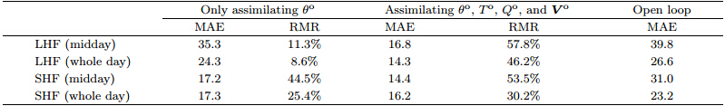
Unlike previous data assimilation experiments usingoff-line LSM simulations, CLS-BLM can be usedto estimate surface heat fluxes and the PBL statesin addition to the soil moisture profile. Sensitivitytests indicate that accurate estimation of surface heatfluxes will require a much shorter assimilation time intervalbecause surface heat fluxes change very quicklyafter sunrise. This rapid adjustment of surface heatfluxes to the diurnal cycle is completely different fromsoil water transfer processes, which occur on a muchslower timescale. Moreover, unlike the backgroundstates, heat fluxes are diagnosed rather than updatedwith each assimilation cycle. Observations only affectheat fluxes indirectly, with gradual adjustments to improvedmodel states. When the update frequency isonce per day, the estimated fluxes are almost identicalto those calculated by the open loop simulation. Theestimated fluxes are still not significantly better thanthe open loop estimates when the assimilation time intervalis reduced to 6 h. The estimated fluxes are onlysubstantially improved when the assimilation time interval is reduced to 0.5 h(Fig. 2). This improvementis especially apparent in the sensible heat flux.Data assimilation improves the estimates more slowlyat later integration times due to the convergence ofthe ensemble members, with data assimilation estimatesof the sensible heat flux at the longest integrationtimes even slightly worse than the open loopresults. The maximum absolute error of the estimatedfluxes during the 15-day data assimilation period alwaysappears at approximately midday, between 1000 and 1600 LT(local time). On average, the largestreduction in MAE lies in the estimates of surface sensibleheat flux. The RMR for sensible heat flux relativeto the open loop flux is 44.5% at midday and 25.4% for the whole day(Table 2). The estimatedlatent heat flux is progressively improved throughoutthe 15-day data assimilation period(Fig. 2a). Thisimprovement may be attributable to simultaneous improvementsin soil moisture estimates, which controlthe surface evaporation when the soil is very dry(asit is in this case). The next subsection will show thatestimates of the surface heat fluxes(especially latentheat flux)can be improved still further when additionalsurface observations are assimilated.
 |
| Fig. 2. Absolute errors(AE)in(a)latent heat flux and (b)sensible heat flux relative to the true fluxes when only θ° isassimilated at an assimilation time interval of 0.5 h(dashed line). The absolute errors for the open loop fluxes are alsoshown(solid line). |
This data assimilation experiment offers no improvementover the open loop ensemble for estimatedprofiles of temperature, humidity, and wind in thePBL, even when the assimilation time interval is reducedto 0.5 h(figure omitted). This result suggeststhat assimilation of θ° alone offers little potential forimproving estimates of the PBL state.4.2 Results from assimilating all observations
This subsection describes an extension of the experimentsdiscussed in Subsection 4.1, in which all observations(i.e., θ°, T°, Q°, and V°)are assimilatedinto CLS-BLM. Consistency with the observationalfrequency(i.e., once every 6 h)at the conventional meteorologicalobservation stations is assured by initiallyadopting a 6-h assimilation time interval. A 0.5-h timeinterval is also used for comparison with the results reportedin Subsection 4.1. Figure 3 shows average soilmoisture estimates in the four specified layers with anassimilation time interval of 6 h. The results obtainedfrom assimilating only θ° and the open loop simulationsof soil moisture are included for comparison. Theestimates of soil moisture when all observations are assimilatedare almost the same as those obtained whenonly θ° is assimilated, although the former are slightlymore consistent with the true soil moisture. This resultimplies that assimilating T°, Q°, and V° does notsubstantially improve estimates of soil moisture, confirmingthat the largest contribution to improvementsin simulated soil moisture profiles comes from assimilatingθ°. This inference is supported by an additionalexperiment in which only T°, Q°, and V° are assimilated.In this case, the estimates are only slightlybetter than the open loop soil moisture(figure omitted).
 |
| Fig. 3. As in Fig. 1, but for experiments assimilating different sets of observations. SM indicates that only θo isassimilated while AO indicates that all observations are assimilated. |
Similar to the experiment in which only θ° is assimilated, the estimated surface heat fluxes are notimproved relative to the open loop fluxes if the assimilationtime interval is set to 6 h(figure omitted).By contrast, reducing the assimilation time interval to0.5 h results in substantial improvements in the estimatedsurface heat fluxes relative to both the θ°-only and open loop experiments, particularly around midday(Fig. 4). Assimilating surface observations leadsto particularly large improvements(i.e., reductions inMAE)in the latent heat flux, with an RMR of 57.8%at midday and an RMR of 46.2% for the whole day(Table 2). Estimates of sensible heat flux are also improvedrelative to the experiment in which only θ° isassimilated(c.f., Fig. 2).
 |
| Fig. 4. As in Fig. 2, but for the experiment in which all observations are assimilated. |
The improvement in PBL state profiles after assimilatingall observations is investigated using theMAE over the full 15-day period because the PBLstate changes often. Four representative times(0800, 1400, 2000, and 0200 LT)are chosen to reflect the diurnalevolution of the PBL structure.
Unlike when only θ° is assimilated, estimates ofpotential temperature profiles are improved relative tothe open loop simulations when all observations are assimilatedon 6-h interval(Fig. 5). These estimates canbe improved still further(especially at low levels)byreducing the assimilation time interval to 0.5 h. Assimilatingall observations even yields improvementsthroughout the profile at night, when the coupling between the surface layer and the upper residual layerbecomes small(Figs. 5c and 5d). Turbulent fluxesweaken at night, while the model lacks the advectivetendency that forces ensemble members to respondto external changes. Accordingly, the ensemble meanchanges little with time. On the other h and , usefulinformation about the daytime state propagates intothe residual layer at nighttime. These two factors mayboth contribute to the skill in estimates of nighttimePBL temperature profiles.
 |
| Fig. 5. Vertical profiles of MAE in potential temperature at(a)0800, (b)1400, (c)2000, and (d)0200 LT averaged overthe 15-day analysis period for experiments in which all observations are assimilated at intervals of 0.5 h(dash-dottedline) and 6 h(dotted line). Results from the open loop simulation(solid line)are also shown. |
The improvements in specific humidity profiles(Fig. 6)are similar to the improvements in temperatureprofiles. The MAE throughout the humidityprofile is reduced relative to the open loop simulationat all four representative times. Furthermore, theMAE is smaller when the assimilation time interval isshorter. Unlike the temperature profiles, the MAE inspecific humidity changes smoothly in the vertical directionwith similar improvements at all levels. Thereason for this is that the ensemble means and incrementsof humidity all change smoothly with height.
 |
| Fig. 6. As in Fig. 5, but for specific humidity. |
Improvements in the profile of horizontal wind(Fig. 7)are also similar to improvements in both temperature and humidity profiles. One difference is thatshorter assimilation time interval provides greater improvementsin estimates of horizontal wind than inestimates of temperature or specific humidity in theafternoon and at night. This difference arises becausethe state of PBL winds often changes quickly in theafternoon while the state at night relaxes gradually towardthe geostrophic wind, resulting in a rapid growthof internal errors. Increasing the frequency of updateshelps to prevent error growth and improve the estimates.
 |
| Fig. 7. As in Fig. 5, but for horizontal wind speed. |
The results of the previous two subsections are allbased on the assumption of specified observational errors(STDs of 1 K for T°, 0.8 g kg−1 for Q°, 1.4 m s−1for |V°|, and 0.03 m3 m−3 for θ°). These experimentsare henceforth referred to as the base-case assimilationexperiments. Observational errors are likely to changein real applications. To investigate the potential impactsof changes in observational errors on the skillof soil moisture, heat flux and PBL state profile estimates, two additional data assimilation experimentsare conducted. Observational errors are reduced by afactor of 5 in the first experiment(errors in soil moistureare reduced by a factor of 3 to 0.01 m3 m−3) and increased by a factor of 5 in the second(errors in soilmoisture are increased to 0.05 m3 m−3).
Estimates of soil moisture profile are severely affectedwhen observational errors are increased, evenbecoming worse than open loop soil moisture at thetwo deepest layers after a few days(figure omitted).The effects on estimates of the PBL potential temperatureprofile are dependent on the time of day(Fig. 8). Improvements relative to the open loop simulationare only evident at 1400 LT. These improvements arerelated to increased ensemble spread at the observinglocation due to strong turbulent mixing. The observedtemperature in the surface layer is highly correlatedwith temperature in the well-mixed PBL at this time, resulting in large analysis increments. At all othertimes(i.e., 0800, 2000, and 0200 LT), the state estimatesare slightly worse than the open loop simulationat some levels because of the smallness of the analysisincrements. The specific humidity profile(Fig. 9)isonly worse than the open loop simulation at a few levelsat 0800 LT. At all other times, the data assimilationstill adds skill due to slow reductions in the ensemblespread. Unlike temperature and humidity, the profileof horizontal wind is still improved relative to the openloop at all levels and all times, although the degree ofimprovement is different at different times(Fig. 10).The winds are always forced by the geostrophic winddistribution, so even at night the ensemble spread doesnot often become small.
 |
| Fig. 8. Profiles of MAE in temperature estimates at(a)0800, (b)1400, (c)2000, and (d)0200 LT using differentranges of observational errors. R1(dashed line)indicates the experiment with smaller observational errors, R2(dashdottedline)indicates the base-case experiment, and R3(dotted line)indicates the experiment with larger observationalerrors. |
 |
| Fig. 9. As in Fig. 8, but for specific humidity. |
 |
| Fig. 10. As in Fig. 8, but for horizontal wind speed |
When the observational errors are specified to besmaller than in the base-case experiment(i.e., a closerfit to the true state), estimates of soil moisture near theobserving location are generally improved relative tothe base-case experiment. The one exception is in thetwo deepest layers, where small ensemble spread leadsto slightly worse estimates at later times(figure omitted).All three PBL state profiles improve consistentlyat all levels relative to the base-case experiment at0800, 1400, and 2000 LT. At upper levels at 0200 LT, temperature estimates do not improve with reductionsin observational errors, while wind estimates even becomeslightly worse than the base-case(although thedegree of deterioration is relatively weak). These resultsindicate that the EnSRF assimilation systemis very sensitive to increases in observational errors and moderately sensitive to decreases in observationalerrors.5. Summary and discussion
An observing system simulation experiment(OSSE)has been designed and carried out to showthe ability of data assimilation to improve estimatesof the soil moisture profile, surface heat fluxes, and PBL states when different sets of observations are assimilated.The coupled l and surface-boundary layer model is a 1D column model with the same PBL parameterizationas the WRF model, forced by WRFforecasts. The EnSRF data assimilation algorithm isused. EnSRF does not require perturbed observations and can provide estimates of anisotropic and inhomogeneousbackground error covariance. The skill of thedata assimilation experiments is quantified on a onepoint scale relative to the true state and open loopsimulations during 13–29 August 2003.
The soil moisture profile can be retrieved effectivelywhen a 6-h assimilation time interval is used, regardless of whether the assimilation includes onlysoil moisture(θ°)or all observations(To, Qo, V o, and θ°). The results are slightly better when all observationsare assimilated. Soil moisture in the deep layercannot be correctly estimated when the assimilationtime interval is 24 h. This result contrasts with theresults of previous studies that used an off-line l and surface model driven by external atmospheric forcings.
Surface heat flux estimates are only substantiallyimproved when the assimilation time interval is furtherreduced from 6 to 0.5 h, with large reductions inMAE between 1000 and 1600 LT. Surface heat fluxesare better when all observations are assimilated thanwhen only θ° is assimilated. These improvements areespecially significant for estimates of the latent heatflux at midday.
Estimates of the PBL state cannot be substantiallyimproved relative to the open loop simulationwhen only θ° is assimilated, even when the assimilationtime interval is reduced to 0.5 h. However, assimilating all observations yields improvements inestimates of the PBL state when the assimilation timeinterval is 6 h, even at night. Reducing the assimilationtime interval to 0.5 h further enhances theaccuracy of estimates of the PBL state. Differences inthe timescales of related processes lead to differencesin the minimum assimilation time interval requiredto improve estimates of soil moisture profiles, surfaceheat fluxes, and PBL state profiles.
Sensitivity tests show that increasing the specifiedobservational errors worsens estimates of deep-layersoil moisture and the vertical structure of the PBLtemperature profile. These estimates are sensitive toincreases in observational errors. Reducing the observationalerrors generally improves the skill of stateestimates near the observing locations, although temperature and wind estimates at upper levels(whichare farther from the observing locations)may worsenslightly at night. This adverse effect is not serious.
Although these results are promising, further researchis needed to successfully apply these assimilationtechniques to real observations. The experimentalcase presented here is limited to a short periodin summer, when horizontal advection is weak and the coupling between the surface and the atmospherealoft is strong. A column model with no advectionmay not provide a correct background forecast for usein EnSRF during winter, when strong advection exists.The most difficult issue when assimilating real observationaldata is how to address model errors fromdifferent sources(e.g., parameterizations of verticaldiffusion and turbulent mixing in the PBL, uncertaintiesin modeling the strength of l and -atmosphericcoupling and feedbacks on local and regional scales, etc.). Model errors may be further complicated whenthe l and surface is heterogeneous. Although EnSRFpotentially has the ability to simultaneously estimateboth model states and model uncertainties using thestate augmentation technique, initial experimentationalong these lines has not been encouraging. More researchis still needed to evaluate this approach dueto the highly nonlinear relationships between modelstates and parameters.
Acknowledgments. Three anonymous reviewersare thanked for insightful comments and suggestions.The language editor for this manuscript is Dr.Jonathon S. Wright.
| [1] | Boussetta, S., T. Koike, K. Yang, et al., 2008: Development of a coupled land-atmosphere satellite data assimilation system for improved local atmospheric simulations. Remote Sens. Environ., 112(3), 720-734. |
| [2] | Chen, F., and J. Dudhia, 2001: Coupling an advanced land surface-hydrology model with the Penn state-NCAR MM5 modeling system. Part I: model implementation and sensitivity. Mon. Wea. Rev., 129, 569-585. |
| [3] | Crow, W. T., and M. J. Van den Berg, 2010: An improved approach for estimating observation and model error parameters in soil moisture data assimilation. Water Resour. Res., 46, W12519, doi:10.1029/2010WR009402. |
| [4] | Ek, M. B., K. E. Mitchell, L. Yin, at al., 2003: Implementation of Noah land surface model advances in the National Centers for Environmental Prediction operational mesoscale Eta model. J. Geophys. Res., 108, D22, doi:10.1029/2002JD003296. |
| [5] | Hacker, J. P., and C. Snyder, 2005: Ensemble Kalman filter assimilation of fixed screen-height observations in a parameterized PBL. Mon. Wea. Rev., 133, 3260-3275. |
| [6] | ——, and D. Rostkier-Edelstein, 2007: PBL state estimation with surface observations, a column model, and an ensemble filter. Mon. Wea. Rev., 135, 2958-2972. |
| [7] | Hess, R., 2001: Assimilation of screen-level observations by variational soil moisture analysis. Meteor. Atmos. Phys., 77, 145-154. |
| [8] | Janjić, Z. I., J. P. Gerrity, and S. Nickovic, 2001: An alternative approach to nonhydrostatic modeling. Mon. Wea. Rev., 129, 1164-1178. |
| [9] | Koster, R. D., Guo Zhichang, Yang Rongqian, et al., 2009: On the nature of soil moisture in land surface models. J. Climate, 22(16), 4322-4335. |
| [10] | Li Xin, Huang Chunlin, Che Tao, et al., 2007: Development of a Chinese land data assimilation system: its progress and prospects. Prog. Nat. Sci., 17(8), 881-892. |
| [11] | Liu Jingmiao, Ding Yuguo, Zhou Xiuji, et al., 2010: A parameterization scheme for regional average runoff over heterogeneous land surface under climatic rainfall forcing. Acta Meteor. Sinica, 24(1), 116-122. |
| [12] | Mahfouf, J. F., 1991: Analysis of soil moisture from near-surface parameters: A feasibility study. J. Appl. Meteor., 30, 1534-1547. |
| [13] | Margulis, S. A., and D. Entekhabi, 2003: Variational assimilation of radiometric surface temperature and reference-level micrometeorology into a model of the atmospheric boundary layer and land surface. Mon. Wea. Rev., 131, 1272-1288. |
| [14] | Niu, G.-Y., Z.-L. Yang, K. E. Mitchell, et al., 2011: The community Noah land surface model with multiparameterization options (Noah-MP): 1. Model description and evaluation with local-scale measurements. J. Geophys. Res., 116, D12109, doi:10.1029/2010JD015139. |
| [15] | Pagowski, M., J. Hacker, and J.-W. Bao, 2005: Behavior of WRF PBL schemes and land-surface models in 1D simulations during BAMEX. Joint WRF/MM5 Users' Workshop, Boulder CO, July 2005, available at http://www.mmm.ucar.edu/wrf/users/workshops/WS2005/ WorkshopPapers.htm. |
| [16] | ——, S. V. Kumar, S. P. P. Mahanama, et al., 2010: Assimilation of satellite-derived skin temperature observations into land surface models. J. Hydrometeor., 11, 1103-1122. |
| [17] | Reichle, R. H., D. B. McLaughlin, and D. Entekhabi, 2001: Variational data assimilation of microwave radiobrightness observations for land surface hydrologic applications. IEEE Trans. Geosci. Remote Sens., 39, 1708-1718. |
| [18] | ——, ——, and ——, 2002: Hydrologic data assimilation with the ensemble Kalman filter. Mon. Wea. Rev., 130, 103-114. |
| [19] | ——, J. P. Walker, R. D. Koster, et al., 2002: Extended versus ensemble Kalman filtering for land data assimilation. J. Hydrometeor., 3, 728-740. |
| [19] | —–, S. V. Kumar, S. P. P. Mahanama, et al., 2010: Assimilation of satellite-derived skin temperature observations into land surface models.J. Hydrometeor., 3, 1103–1122. |
| [20] | Rémy, S., and T. Bergot, 2009: Ensemble Kalman filter data assimilation in a 1D numerical model used for fog forecasting. Mon. Wea. Rev., 138(5), 1792-1810. |
| [21] | Ruggiero, F. H., K. D. Sashegyi, R. V. Madala, et al., 1996: The use of surface observations in four-dimensional data assimilation using a mesoscale model. Mon. Wea. Rev., 124, 1018-1033. |
| [22] | Seuffert, G., H. Wilker, P. Viterbo, et al., 2003: Soil moisture analysis combining screen-level parameters and microwave brightness temperature: A test with field data. Geophys. Res. Lett., 30(10), 1498, doi:10.1029/2003GL017128. |
| [23] | Svensson, G., A. A. M. Holtslag, V. Kumar, et al., 2011: Evaluation of the diurnal cycle in the atmospheric boundary layer over land as represented by a variety of single-column models: The second GABLS Experiment. Bound.-Layer Meteor., 140(2), 177-206. |
| [24] | Tian Xiangjun, Xie Zhenghui, and A. Dai, 2008: A land surface soil moisture data assimilation system based on the dual-UKF method and the Community Land Model. J. Geophys. Res., 113, D14127, doi:10.1029/2007JD009650. |
| [25] | Van den Hurk, B., M. Best, P. Dirmeyer, et al., 2011: Acceleration of land surface model development over a decade of GLASS. Bull. Amer. Meteor. Soc., 92(12), 1593-1600. |
| [26] | Walker, J. P., G. R. Willgoose, and J. D. Kalma, 2001: One-dimensional soil moisture profile retrieval by assimilation of near-surface observations: A comparison of retrieval algorithms. Adv. Water Resour., 24, 631-650. |
| [27] | Whitaker, J. S., and T. M. Hamill, 2002: Ensemble data assimilation without perturbed observations. Mon. Wea. Rev., 130, 1913-1924. |
| [28] | Yang Junli and Shen Xueshun, 2010: The construction of SCM in GRAPES and its applications in two field experiment simulations. Adv. Atmos. Sci., 28(3), 534-550. |
| [29] | Yang Yi, Gong Zhongqiang, Wang Jinyan, et al., 2011: Time-expanded sampling approach for ensemble Kalman filter: Experiment assimilation of simulated soundings. Acta Meteor. Sinica, 25(5), 558-567. |
| [30] | Yang, Z.-L., G.-Y. Niu, K. E. Mitchell, et al., 2011: The community Noah land surface model with multiparameterization options (Noah-MP): 2. Evaluation over global river basins. J. Geophys. Res., 116, D12110, doi:10.1029/2010JD015140. |
| [31] | ——, Li Deqin, and Qiu Chongjian, 2011: A multimodel ensemble-based Kalman filter for the retrieval of soil moisture profiles. Adv. Atmos. Sci., 28(1), 195-206. |
| [32] | Zhang Shuwen, Li Haorui, Zhang Weidong, et a1., 2005: Estimating the soil moisture profile by assimilating near-surface observations with the Ensemble Kalman Filter (EnKF). Adv. Atmos. Sci., 22(6), 936-945. |
| [34] | ——, Zhang Weidong, and Qiu Chongjian, 2007: A variational method for estimating near-surface soil moisture and surface heat fluxes. Acta Meteor. Sinica, 21(4), 476-486. |
| [33] | ——, Zeng Xubin, Zhang Weidong, et al., 2010: Revising the ensemble-based Kalman Filter covariance for the retrieval of deep-layer soil moisture. J. Hydrometeor., 11(1), 219-227. |
| [34] | —–, Li Deqin, and Qiu Chongjian, 2011: A multimodel ensemble-based Kalman filter for the retrieval of soil moisture profiles.Adv. Atmos. Sci., 28(1), 195–206. |
| [35] | Zhou Yuhua, D. McLaughlin, and D. Entekhabi, 2006: Assessing the performance of the ensemble Kalman filter for land surface data assimilation. Mon. Wea. Rev., 134(8), 2128-2142. |