 2013, Vol. 27
The Chinese Meteorological Society
Article Information
- WAN Wei, LI Huang, CHEN Xiuwan, LUO Peng, WAN Jiahuan. 2013.
- Preliminary Calibration of GPS Signals and Its Effects on Soil Moisture Estimation
- J. Meteor. Res., 27(2): 221-232
- http://dx.doi.org/10.1007/s13351-013-0207-7
-
Article History
- Received July 18, 2012
- in final form December 10, 2012


2. Meteorological Observation Center of China Meteorological Administration, Beijing 100081;
3. 92292 Troops PLA, Qingdao 266405
The versatile refracted, reflected, and scatteredsignals of the Global Navigation Satellite Systems(GNSS)have been successfully utilized to sound theatmosphere and ionosphere, ocean, l and surface, and the cryosphere. The L-b and microwave signal withpretty high temporal resolution from the GNSS satellite becomes a new source of remote sensing data. TheGNSS Reflectometry(GNSS-R)involves measurementof reflections from the earth of navigation signals, and it has already shown its potential in earth observationover different kinds of surfaces(Liu et al., 2007).
Soil moisture content(SMC)is a key componentof the water cycle, and it influences the sensible and latent heat flux from l and surface to the atmosphere(Zhang et al., 2007). Many types of traditional remotesensors have been used to sense SMC. Data gatheredvia satellite remote sensing provide consistent measurement of soil moisture on the global scale, but thesedata are high-cost because of the required equipment(Larson et al., 2008; Yan et al., 2011). SMC estimationusing GNSS-R technique is relatively low-cost since wecan acquire reflected data from GNSS satellites at nocharge as long as we have receivers. In addition, similar to other L-b and active microwave sensors, GNSS-Rhas the possibility of day/night operations in all sortsof weather conditions(Wan et al., 2012a). The GNSSderived signal is influenced most strongly by nearsurface(0-5 cm)soil moisture, similar to those ofthe ESA(European Space Agency)Soil Moisture and Ocean Salinity(SMOS)mission and the NASA's SoilMoisture Active Passive(SMAP)mission. Global Positioning System(GPS)is one of the most popularsystems for navigation, which makes it a frequentlyused signal generator for SMC estimation. In order toimprove the estimation accuracy, both the direct and reflected GPS signals need to be calibrated to eliminate the signal error.
Many researchers have been working on estimation of SMC using GNSS-R technique. Masters et al.(2004)demonstrated the capability of this techniqueto obtain signal to noise ratios(SNR), which are highenough to sense small changes in surface reflectivity.Mao et al.(2009) and Wang et al.(2009a)both conducted some validations between GPS reflected power and the in-situ SMC. The SNR data derived from traditional single-antenna GPS receiver and its relationto bare soil moisture were discussed by Larson et al.(2008, 2010). Zavorotny et al.(2010)built a physical model using GPS SNR data for bare soil moistureretrieval. Rodriguez-Alvarez et al.(2010)proposeda GPS data-based method called Interference PatternTechnique(IPT)to sense SMC, and they used a newinstrument named Soil Moisture Interference-patternGNSS Observations at L-b and (SMIGOL)reflectometer. Song et al.(2007) and Wang et al.(2009b)both made some attempts to establish models withbistatic-radar equations. Zhang and Yan(2009)explored simulations of reflection waveforms and estimations of SMC. However, all the above studies did nottake the calibration of GPS signals into consideration.Katzberg et al.(2005)reported the first calibration ofreflected GPS signals using an over-water method and estimation of surface dielectric constant compared tosurface truth. Yan et al.(2011)used wavelet methodto remove the high frequency noise existing in the direct signals of GPS.
This paper presents a follow-on or an expansionof the earlier work by Katzberg et al.(2005), related to the calibration of GPS signals. We introducethe Polynomial fitting method and over-water methodto calibrate direct and reflected signals of GPS satellites. These two methods were proposed previouslyby Katzberg et al.(2005), but they did not give detailed explanation about the theoretical basis for suchalgorithms, and they did not quantitatively analyzehow and how much the signal calibration could affectthe SMC estimation either. The aim of this study isto provide the theoretical basis for the two calibrationmethods proposed previously and to give some furtherdiscussion on the calibration effects. We use data fromthe Soil Moisture Experiments in 2002(SMEX02)forvalidation just as Katzberg et al.(2005)did before.Errors of sites with different Normalized DifferenceVegetation Indices(NDVIs)are calculated, and theeffects of calibration on estimation of soil reflectivity and dielectric constant are evaluated. Furthermore, aiming at making our method suitable for sites withhigh vegetation cover, we subsequently propose a correction factor that considers the vegetation effect inorder to reduce the "over-calibration" over the siteswith thick vegetation.2. SMC estimation model using calibrated signals2.1 Characteristics of GPS surface scattered signal
Figure 1 depicts the bistatic-radar geometry ofa typical GPS satellite to aircraft or ground geometry. The letters t, s, and r refer to transmitter, l and surface, and receiver, respectively. The transmitteris located on a GPS satellite with an orbit altitude of20200 km. The receiver simultaneously measures boththe direct signal and the signal reflected from the earthsurface. The direct signals transmitted by the GPSsatellite are right-h and circularly polarized(RHCP), while for typical incidence, the reflected signals arepredominantly left-h and circularly polarized(LHCP)with very little RHCP components. Therefore, thereceiver commonly has two antennas, one is RHCPfor receiving direct signal and the other is LHCP forgathering surface scattered signal. The specular pointdepicted in Fig. 1 is defined as the point on the surfacewith the minimum bistatic range and for which incidence and reflection angles are equal. The reflectionfollows Fresnel's law in specular points. Equi-rangepoints on the surface form ellipses surrounding thespecular point, which are called the rough surface glistening zone(Masters et al., 2004).
 |
| Fig. 1. The geometry of transmission of GPS surface scattered signal. |
GPS signals make interaction with the earth surface when they pass through the thick atmosphere and finally reach the earth. The phase and amplitudechange along with the effect of surface(soil moisture, snow, etc.). For a perfect flat surface, the specularlyreflected power is coherent and governed by Fresnel'sreflection law. As the surface roughness increases, thecoherent component of the reflected signal decreases, and the incoherent component scattered in other directions increases. In this paper, we only choose thespecular points as our target and ignore the incoherentcomponent since it is too much complicated.2.2 Traditional SMC model
The traditional GPS data-based model for SMCestimation mainly includes three steps: 1)extractingsoil reflectivity from GPS raw data; 2)deducing dielectric constant of soil from the reflectivity; 3)calculatingSMC using dielectric constant. Assume that the powerof direct signal is Pd, the reflected power from soil isPr, and the soil reflectivity is described by
Here, the ratio ofPr and Pd is sometimes called normalized power.
As for specular points, the surface is perfectlysmooth(Choudhury et al., 1979), so the Kirchoff Approximation of reflectivity(Masters et al., 2004)is simplified to
where λ is the glancing angle or elevation angle, and R(λ)is the Fresnel reflection coefficients of the equivalent smooth surface. R(λ)is a combination of horizontal and vertical polarization coefficientss as givenby Ulaby et al.(1987), from which the dielectric constant " is obtained. Once " is obtained, SMC is estimated easily using the semi-empirical model proposedby Topp et al.(1980)or Hallikainen et al.(1985).2.3 Improved model with calibrated signals
As shown in Eq.(1), the traditional model usesthe value of normalized power to represent soil reflectivity. However, this is actually based on the following hypotheses: it is assumed that Rsr is the distancebetween GPS receiver and soil surface, Rts is the distance between transmitter and surface, and Rtr is thedistance between transmitter and receiver(Fig. 1).Rsr is commonly with orders of ~100, ~103, and ~105m for ground-based, airborne, and spaceborne observations, respectively; while Rts and Rtr usually havean order of ~2×10⁷ m. Since we know that Rsr ≤ Rts and Rsr ≤ Rtr, the path difference is ignored in mostcases. That is to say, Pd equals the direct power thatthe soil receives and Pr equals the reflected power fromthe soil. Actually, these two parameters come fromthe receiver not the soil itself. Obviously, it causeserrors when using the above two replacements, especially when it comes to airborne or spaceborne cases.
In addition, the errors of signals received byantennas also include: 1)different multipath effects between "transmitter vs. RHCP antenna" and "transmitter vs. soil"; 2)atmospheric attenuationassociated with reflected signals traveling from soilto LHCP antennas; 3)different properties inherentwith LHCP and RHCP antennas, which lead to differences in measurement of the direct and reflectedpower. Therefore, before the GPS receiver can be usedas official reflector for SMC estimation, both the direct and reflected signals need to be calibrated to eliminatethe signal error. In this study, we introduce the overwater method proposed by Katzberg et al.(2005)tocalibrate reflected signals, and we use a three-orderpolynomial to calibrate direct signals.
A schematic representation of airborne GPS signal calibration is shown in Fig. 2. The two trianglesbeside point A denote the RHCP and LHCP antennas.Points B and C depict specular points of soil and water, respectively. The water reflectivity is consideredas a constant corresponding to the normal-incidence(60°-85°)reflectivity of water at L-b and (Katzberg et al., 2005). Subsequently, the reflected signal is referenced to the over-water calibrated signal using thescale factor determined in this way. More details ofthe calibration method are described as follows:
 |
| Fig. 2. A schematic diagram for airborne GPS signal calibration. |
1)Calibration of direct signals. During the observation period, except for location and status variations of GPS(especially for airborne and spaceborne)receiver, there are many other factors that influencethe direct signal power, such as changes of elevationangle and azimuth angle, and the multipath effect. Inmost cases, it merely takes a couple of hours to finisha GPS-based soil moisture observation, and the directsignal power received by GPS antenna keeps stableduring these hours. Therefore, the only thing we dois to try to fit a polynomial to the dataset of directpower in order to remove the r and om noises. Generally, a three-order polynomial is used to finish thework. We finally convert the original direct power Pdto a calibrated one named P'd.
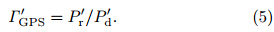
2)Calibration of reflected signals. As mentionedpreviously, we introduce the over-water method to calibrate signals reflected from soil. In any of the airborneor spaceborne observations, it is easy for us to choosea calm water area(e.g., a lake or a pool), which isclose to our soil surface observation. The water area and the soil surface have approximately the same atmosphere condition, reflector height, observation time, and equipment condition. A series of GPS direct and reflected powers are measured and converted to seriesof water reflectivity ΓGPSw using Eq.(1), which are averaged to obtain the mean value of GPS-derived water reflectivity. Moreover, the real water reflectivityΓw is considered as a constant in certain conditionsdiscussed previously. The calibration factor fc for reflected GPS signals is derived by
The calibrated reflected power P'r is expressed asThus, similar to Eq.(1), the calibrated soil reflectivityis expressed as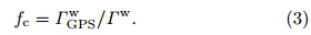

Therefore, the traditional GPS-based SMC modelis finally improved when using Γ'GPS instead of the traditional ΓGPS.3. Calibration process and results
The data we use for model validation come fromthe airborne GPS data of SMEX02. We downloadedthe data from the National Snow and Ice Data Center of the U.S.(NSIDC; http://nsidc.org/daac/). TheSMEX02 experiment was conducted in the Iowa Stateduring June and July 2002 over the intensively sampled sites in the Walnut Creek region south of Ames.
The GPS reflectometer, with its potential applicationto remote sensing of global hydrological cycle, was included in this experiment.The GPS reflectometer was installed on theNCAR HC-130 aircraft. The aircraft flew at an altitude of approximately 1.1 km above the surface withan average speed of 75 m s-1. The direct and reflectedpowers were recorded during the flight on 9 discontinuous days between June 19 and July 8, 2002. Thedata on June 19 were discarded because of equipmentproblems.
The in-situ data were also collected over the Walnut Creek region during the flight period. The samplesites included 10 soybean sites and 21 corn sites, and the collected data contained bulk density, gravimetric and volumetric soil moistures, surface and subsurfacesoil temperatures, etc. The data downloaded from theNSIDC website contain four levels: Level 0, Level 1a, Level 1b, and Level 2, and more detailed informationof these levels is given by Wan et al.(2012b). In thisstudy, we choose data on June 25, 2002 for our modelvalidation purpose, since the data on this day havelarger numbers of points and better quality than onany other day of the flight period.3.1 Signal calibration of SMEX02 data
Figure 3 shows the flight route on 25 June 2002.The yellow lines depict the exact flight route, and the background imagery is L and sat ETM+(EnhancedThematic Mapper Plus)on 23 June. The square(a)shows its track over a lake, whose data obtained areused to calibrate the reflected signals. The square(b)displays a sample region of the flight route over cropfields. More details of the l and surface cover are described in the top-right square of Fig. 3, from whichwe can see the boundaries of each crop field and alsosome bare soil regions and urban areas.
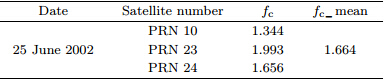
During the observation period, there are threegood tracks of GPS satellites, i.e., PRN10, PRN23, and PRN24, and the elevation angle is between62.12° and 83.39°. According to measurements from Katzberg et al.(2005), water reflectivity of the lakein GPS L1-b and equals 0.63, i.e., Γw = 0:63 in Eq.(3). We use Level 1a product to calculate the calibration factors fc of the three tracks in Eq.(3), and the derived fc for each track is shown in Table 1. InTable 1, the calibration factor of PRN12, PRN23, and PRN24 equals 1.344, 1.993, and 1.656, respectively, with a mean value of 1.664. The fc values we obtainhere are approximately the same as those reported by Katzberg et al.(2005). Meanwhile, we use a threeorder polynomial fitting method to calibrate the directpower of that day. We choose Level 2 product to calculate soil dielectric constant since Level 2 data contain only specularpoints. Denoising process is conducted firstly for thereflected power. The mean noise power Pnoise is givenin the data set, and we use
As described in Iowa Soil Properties and Interpretations Database(ISPAID 6.0), the surface s and content and clay content of soil in the Walnut Creekregion are 0%-80% and 0%-38%, respectively. To simplify the calculation, we use the mean value of s and and clay content of the whole region instead of theirrespective values. In other words, we use S = 28% and C = 27% in the Hallikainen SMC model(Hallikainen et al., 1985), and then derive the volumetric watercontent(VWC)of soil for both Pre-Cal and Post-Calcases. Note that we use VWC to denote SMC in thisstudy. Besides, it should be pointed out that the Hallikainen model is not suitable for estimating SMC ofvery dry soils(ε < 3)(Hallikainen et al., 1985; Yan and Zhang, 2010), and we treat these values as outliers and deliberately remove them before we definethe errors of our estimation.
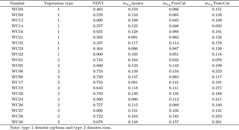
Figure 5 shows distributions of the corn and soybean sites in Walnut Creek. Surface VWC was measured with a Theta Probe(TP), Type ML2. The TPis a manually-operated impedance instrument manufactured by Delta-T Devices, Ltd., Cambridge, Engl and . Surface soil moisture was sampled each morning(8-11 am local time)during the experiment. Fourteen sampling points were collected with the probe being inserted vertically into the soil(0-6 cm)at threepoints along the crop row. Here we use the averagevalue of each site for validation. The average valueis generated from both the samples' average and thevertical depths validation average. We choose 21 sitesfrom all the 31 sites in Fig. 5 since these 21 sites contain specular points, including 9 soybean sites and 12corn sites. Comparisons are shown in Table 2. We alsogive the NDVI values of these sites in Table 2, whichare extracted from L and sat ETM+ imagery. It is obvious that NDVIs of soybeans are lower than those ofcorns. Note that NDVI equals 0 in WC13, WC32, and WC27, which means that these three NDVI points liein ridges or some other kinds of bare soil.
We divide all the 21 rows into 3 catalogs according to the NDVI values: bare soil(NDVI = 0), midvegetation cover(Mid-Veg; 0 < NDVI ≤ 0.6), and high-vegetation cover(High-Veg; NDVI > 0.6), and we use NDVI as an indicator of vegetation cover. Errors of SMC estimation for different vegetation coversare shown in Table 3. It is found that the accuracy ofSMC estimation is highly related to vegetation. Forcases of NDVI = 0 and 0 < NDVI ≤ 0.6, our modelhas derived much better results than the traditionalmodel, with errors of 11.17% and 8.12%, respectively.However, for the sites with NDVI values greater than0.6, the new model achieves even worse results thanthat of Pre-Cal. This is expected as the vegetationeffect in high vegetation site is not considered, and wewill give further discussion in the later section of thispaper.
The differences of soil reflectivity between Pre-Cal and Post-Cal are shown in Figs. 6a and 6b. Figure 6a describes the soil reflectivity of PRN 24 between 14:24:00 and 15:22:02 UTC(hh:mm:ss), and Fig. 6b shows PRN10 between 15:22:14 and 16:48:00UTC. Red points indicate Pre-Cal and blue points indicate Post-Cal. As a whole, the Post-Cal reflectivityis higher than that of Pre-Cal. This is because ourcalibration coefficients fc is greater than 1. The mostdirect effect of higher soil reflectivity values is thatthey lead to higher dielectric constant values. Theoretically, the estimated SMC values become higherafter calibration, and this is in accordance with theresults in Table 2.
Figure 7 illustrates the relationship between estimated ε of Post-Cal and the in-situ soil moisturecollected by TP. Soybeans are depicted in hollow triangles and corns in solid squares. We also draw theestimated SMC values of Post-Cal using red plus signsin Fig. 7. The SMC estimation using the calibratedmodel shows either higher or lower values, comparedwith in-situ observations, with 5:4 a ratio of numbersfor soybean and 10:2 for corn. It is not difficult todiscern the causes of this: in bare soil or Mid-Vegsites, our estimated SMC is lower than that of insitu values in most cases, and after we multiply thereflected power with fc, those estimated SMC valuesfinally turn into two different cases, i.e., higher thanin-situ or still lower than in-situ, and all these dependon the values of fc. Note that the SMC estimationsin High-Veg sites are higher than their correspondingin-situ values even in Pre-Cal cases, and there is nodoubt that they are far above in-situ values after calibration. Therefore, vegetation effect is supposed tobe considered in High-Veg sites so as to remove the"over-calibration" phenomenon.
Two typical sites of soybean and corn are shownin Fig. 8. Figure 8a is WC09 with soybean and Fig. 8b is WC06 with corn. These two figures illustratevegetation differences of the two kinds of crops. Soybean is in its initial period of growth while corn ismostly in the middle period. Vegetation coverage ismuch thicker in WC06 than that in WC09. Comparisons between estimated SMC values(including PreCal and Post-Cal) and the in-situ values are shown inFigs. 9a and 9b. Note that corn sites exhibit muchnosier results than the soybean sites because of theirthicker vegetation cover. For further comparison, Figs.10a and 10b show the Ratio-Point-Clusters of SMCestimations(Post-Cal) and the in-situ observations.Note that the "over-calibration" appears to be moreserious in Fig. 10b than in Fig. 10a.
According to the above analysis, the reflectionof vegetation leads to deterioration of the calibratedSMC model, especially for sites with high vegetationcover. Ulaby et al.(1987)figured out that attenuation occurs when the reflected microwave signals of soiltravel through vegetation, and this causes the inaccurate soil moisture retrieval. In this study, the GPSLHCP antenna receives fewer signals over the highNDVI site. In High-Veg sites, Eq.(3)actually ignores the effect of reflection from vegetation; instead, it treats the total power of both soil and vegetation asthe reflection of soil itself, and this is the exact reasonfor "over-calibration". Therefore, we propose a factorcalled Vc in order to modify the calibration coefficientsfc.
In Eq.(4), the reflected power Pr is modified toP''r when adding Vc into the equation:
Here, we treat the change of NDVI as linear, and we modify the increment of fc to obtain the expressionof Vc:
Come back to Table 2, we recalculate SMC valuesfor all the 12 sites with NDVI > 0.6: here, after sometrials, a = 0.8 is defined as the best value of coefficientsa, and f'c is used instead of fc in Eq.(6)in order toderive a modified reflected power. Figure 11 depictsa comparison between estimated SMC(after modification of fc) and the in-situ value. Compared to Fig. 9b, it is obvious that a better SMC estimation is obtained after modification of the calibration coefficients.Note that there are still two sites(WC01 and WC08)with large errors, and this is because the reflectivitymeasured by GPS is too low. Figure 12 shows theRatio-Point-Cluster of estimated SMC(after modification of fc) and the in-situ observation, from whichthe comparison of the values before and after modification can be discerned more directly. We finally achievean error of 3.81% in the above-mentioned High-Vegsites in Table 3, and this error is lower than that ofthe calibrated model(52.62%)as well as that of thetraditional model(8.92%). We even consider to further improve the Vc calculation in order to make itmore flexible in our next work.
This study has shown that calibration of GPSsignal is an important step that should be consideredbefore using the GPS-derived data to estimate surface soil moisture. Methods of GPS signal calibrationinvolving both the direct and reflected signals havebeen introduced, and a detailed explanation of thetheoretical basis for such algorithms has been given.Further relationships of GPS reflectivity to soil dielectric constant and to SMC have been investigated, and an improved model using calibrated signals has beenestablished. It is shown that the calibrated modelderives better results than the traditional model under bare soil or Mid-Veg conditions. For High-Vegsites, the effect of signal attenuation due to vegetationcover has been preliminarily taken into consideration, and a linear model related to NDVI has been established to derive a correction factor for reducing the"over-calibration" problem. While these results areencouraging, further study is needed to determine amore flexible vegetation-modifing factor using radiative transfer equations and biomass parameters(e.g., vegetation height and vegetation water content). Inaddition, we used the semi-empirical relationships developed by Hallikainen et al.(1985)in this study. Oneof the limitations of such a dielectric model is that itis hard to estimate SMC of very dry soils. More advanced models have been proposed, which account forbound soil water(e.g., Mironov et al., 2004), and itwould be instructive to verify these new models usingthe GPS-derived data.
Acknowledgments: We would like to thankNSIDC for providing the SMEX02 data. We appreciate Dr. Zhao Limin from the Institute of RemoteSensing Applications, Chinese Academy of Sciences, and Dr. Xiao Han from Peking University for theirgreat suggestions. We are also grateful to the anonymous reviewers and editors for their helpful comments.

Fig. 3. The °ight route on 25 June 2002. 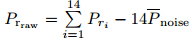 to derive the total power Prraw of all the 14 reflectionchannels, which is then defined a raw power after denoising but before calibration. We use Eq.(4) and thefc values in Table 1 to derive soil reflectivity Γ'GPS. Finally, we use the method proposed by Zavorotny and Voronovich(2000)to calculate the soil dielectric constants ε. In order to compare the differences with and without calibration, we also calculate the soil dielectric constants using the raw direct and reflected power, respectively. The derived ε values in both cases areshown in Figs. 4a and 4b. Figure 4a denotes thedistribution of " using pre-calibration(Pre-Cal)data, while Fig. 4b denotes " using post-calibration(Post-Cal)data. As shown in these two figures, we divideε into different catalogs according to their values, and the Post-Cal gets four catalogs while the Pre-Cal getsonly three, missing a catalog of "28.0-69.0". A moredetailed comparison between the two is shown in Fig. 4c, and it is clear that signal calibration makes ε ahigher value as it was supposed to be.
Fig. 4. Comparison of ε between Pre-Cal and Post-Cal.(a)ε of Pre-Cal, (b)ε of Post-Cal, and (c)comparison between the two. 
Fig. 5. Distributions of corn and soybean sites in Walnut Creek. Soybean is in green and corn in yellow. 
Fig. 6. Comparison of reflectivity between Pre-Cal and Post-Cal.(a)PRN24;(b)PRN10. 
Fig. 7. Relationship among estimated ε of Post-Cal, in-situ soil moisture collected by TP, and estimated SMCvalues of Post-Cal. 
Fig. 8. Differences of vegetation cover between(a)soybean sites and (b)corn sites. 
Fig. 9. Comparison between SMC estimations(including Pre-Cal and Post-Cal) and the in-situ observations over(a)soybean sites and (b)corn sites. 
Fig. 10. Ratio-Point-Cluster of SMC estimations(Post-Cal) and the in-situ observations over(a)soybean sites and (b)corn sites. 
Fig. 11. Comparison between the SMC estimation(after modification of fc) and the in-situ observation. 
Fig. 12. Ratio-Point-Cluster of the SMC estimation(after modification of fc) and the in-situ observation.


| [1] | Choudhury, B., T. Schmugge, and A. Chang, 1979: Effect of surface roughness on the microwave emission from soils. J. Geophys. Res., 84(C9), 5699-5706. |
| [2] | Hallikainen, M. T., F. T. Ulaby, M. C. Dobson, et al., 1985: Microwave dielectric behavior of wet soil. Part I: Empirical models and experimental observations. IEEE Trans. Geosci. Remote Sens., GE-23(1), 25-34. |
| [3] | Katzberg, S. J., O. Torres, M. S. Grant, et al., 2005: Utilizing calibrated GPS reflected signals to estimate soil reflectivity and dielectric constant: Results from SMEX02. Remote Sens. Environ., 100, 17-28. |
| [4] | Larson, K. M., E. E. Small, E. D. Gutmann, et al., 2008: Using GPS multipath to measure soil moisture fluctuations: Initial results. GPS Solut., 12(3), 173-177. |
| [5] | —, J. J. Braun, E. E. Small, et al., 2010: GPS multipath and its relation to near-surface soil moisture content. IEEE J-STARS, 3(1), 91-99. |
| [6] | Liu Jingnan, Shao Lianjun, and Zhang Xunxie, 2007: Advances in GNSS-R studies and key technologies. Geomatics and Information Sci. of Wuhan Univ., 32(11), 955-960. (in Chinese) |
| [7] | Mao Kebiao, Wang Jianming, Zhang Mengyang, et al., 2009: The study of soil moisture retrieval from GNSS-R signals based on AIEM model and experiment data. High Tech. Lett., 19(3), 295-301. (in Chinese) |
| [8] | Masters, D., P. Axelrad, and S. Katzberg, 2004: Initial results of land-reflected GPS bistatic radar measurements in SMEX02. Remote Sens. Environ., 92, 507-520. |
| [9] | Mironov, V. L., M. C. Dobson, V. H. Kaupp, et al., 2004: Generalized refractive mixing dielectric model for moist soils. IEEE Trans. Geosci. Remote Sens., 42(4), 773-785. |
| [10] | Rodriguez-Alvarez, N., A. Camps, M. Vall-Llossera, et al., 2010: Land geophysical parameters retrieval using the interference pattern GNSS-R technique. IEEE Trans. Geosci. Remote Sens., 49(1), 71-84. |
| [11] | Song Dongsheng, Zhao Kai, and Guan Zhi, 2007: Soil moisture retrieval using airborne GNSS-R technology. J. Northeast Forestry Univ., 35(5), 94-96. (in Chinese) |
| [12] | Topp, G. C., J. L. Davis, and A. P. Annan, 1980: Electromagnetic determination of soil water content: Measurements in coaxial transmission lines. Water Resour. Res., 16(3), 574-582. |
| [13] | Ulaby, F. T., R. K. Moore, and A. Fung, 1987: Microwave Remote Sensing: Active and Passive (Vol. 3). Aztech House, Michigan, 1846-1850. |
| [14] | Wan Wei, Chen Xiuwan, Li Guoping, et al., 2012a: GNSS Reflectometry: A review of theories and empirical applications in ocean and land surfaces. Remote Sens. Information, 27(3), 117-123. (in Chinese) |
| [15] | —, Chen Xiuwan, Luo Peng, et al., 2012b: Analysis of airborne GPS reflected data of SMEX02. Remote Sens. Information, 27(6), 127-133. (in Chinese) |
| [16] | Wang Yingqiang, Yan Wei, Fu Yang, et al., 2009a: Soil moisture measuring based on airborne GPS reflectometry. J. Remote Sens., 13(4), 678-685. (in Chinese) |
| [17] | Wang Yan, Yang Dongkai, Hu Guoying, et al., 2009b: Sensing of the soil moisture using GPS-reflected signals. GNSS World of China, 5, 7-10. (in Chinese) |
| [18] | Yan Songhua and Zhang Xunxie, 2010: Retrieving soil moisture based on GNSS-R signals. Chinese J. Radio Sci., 1, 8-13. (in Chinese) |
| [19] | —, Gong Jianya, Zhang Xunxie, et al., 2011: Ground based GNSS-R observations for soil moisture. Chinese J. Geophys., 54(11), 2735-2744. (in Chinese) |
| [20] | Zavorotny, V. U., and A. G. Voronovich, 2000: Scattering of GPS signals from the ocean with wind remote sensing application. IEEE Trans. Geosci. Remote Sens., 38(2), 951-964. |
| [21] | —, K. M. Larson, J. J. Braun, et al., 2010: A physical model for GPS multipath caused by land reflections: Toward bare soil moisture retrievals. IEEE J-STARS, 3(1), 100-110. |
| [22] | Zhang Shuwen, Qiu Chongjian, and Zhang Weidong, 2007: Estimates of surface heat fluxes and nearsurface soil moisture using a variational method. Acta Meteor. Sinica, 65(3), 440-449. (in Chinese) |
| [23] | Zhang Xunxie and Yan Songhua, 2009: Moisture estimation using GPS reflected signals. GNSS World of China, 3, 1-6. (in Chinese) |