 2013, Vol. 27
The Chinese Meteorological Society
Article Information
- Guo Jianping, Niu Tao, Pooyan Rahimy, WANG Fu, ZHAO Haiying and ZHANG Jiahua. 2013.
- Assessment of Soil Erosion Susceptibility Using Empirical Modeling
- J. Meteor. Res., 27(1): 98-109
- http://dx.doi.org/10.1007/s13351-013-0110-2
-
Article History
- Received March 27, 2012
- in final form September 22, 2012


2 Institute of Geo-Information Science and Earth Observation of the University of Twente, 7500 AA Enschede, the Netherlands;
3 School of Resources and Environment, University of Electronic Science and Technology of China, Chengdu 611731, China;
4 Shanxi Meteorological Observatory, Taiyuan 030006, China;
5 Center for Earth Observation and Digital Earth, Chinese Academy of Sciences, Beijing 100094, China
The soil loss estimated from the modified RUSLE model shows a large spatial variance, ranging from 10 to as much as 7000 ton ha−1 yr−1. The high erosion susceptible area constitutes about 46.8% of the total erosion area, and when classified by land cover type, 33% is “mixed bare with shrubs and grass”, followed by 5.29% of “mixture of shrubs and trees”, with “shrubs” having the lowest percentage of 0.06%. In terms of slope types, very steep slope accounts for a total of 40.90% and belongs to high susceptibility, whereas flat slope accounts for only 0.12%, indicating that flat topography has little effect on the erosion hazard. As far as the geomorphologic types are concerned, the type of “moderate steep–steep slopes with moderate to severe erosion” is most favorable to high soil erosion, which comprises about 9.34%.
Finally, we validate the soil erosion map from the adapted RUSLE model against the visual interpretation map, and find a similarity degree of 71.9%, reflecting the efficiency of the adapted RUSLE model in mapping the soil erosion in this study area.
Soil erosion is a hazard traditionally associatedwith agriculture in the tropical and semi-arid areas and has great long-term effects on soil productivity and sustainable agriculture(Morgan, 1995). Soil erosionis correlated with about 85% of l and degradationin the world, leading to up to 17% reduction in cropproductivity(Oldeman et al., 1990). To exactly assessthe soil erosion is still challenging, partly due to thediverse factors affecting the estimation of soil erosion, especially due to the anthropologic activities. Generally, there are two approaches to assess the soil erosionsusceptibility, i.e., the qualitative method(visual imageinterpretation) and the quantitative method(erosionmodels). Besides the visual interpretation of soilerosion from satellite images or aerial photographs, alarge number of erosion models exist, which can be dividedinto empirical models and physical-based models(Morgan, 1995). Empirical models have a statisticalbasis, whereas physical-based models intend todescribe the controlling processes on a storm eventbasis. Nevertheless, many models contain both empirical and physically based components. Recent reviewsof several state-of-the-art erosion models are given by Merritt et al.(2003) and Vrieling(2006).
Compared with the traditional field measurementsof soil erosion, remotely sensed data can greatlyimprove the erosion mapping through direct erosiondetection or through the use of erosion controlling factors.The intermediate parameter, like NormalizedDifference Vegetation Index(NDVI), is a good example, which is one of the key input parameters forthe empirical models. Also, satellite imagery has thepotential to provide regional spatial data for severalinput parameters to erosion models(e.g., King and Delpont, 1993; Pelletier, 1985). Furthermore, the automaticextraction of eroded l and s from satellite imageryis a sound alternative for visual interpretationtechniques. For instance, Servenay and Prat(2003)applied an unsupervised classification algorithm tomultispectral SPOT(Syst´eme Pour l’Observation dela Terre)HRV(High Resolution Visible)data to distinguishfour stages of erosion.
The most widely used model is the UniversalSoil Loss Equation(USLE), which is an empiricalmodel assessing long-term averages of sheet and rillerosion, based on plot data collected in eastern USA(Wischmeier and Smith, 1978). The USLE and itsadapted versions, i.e., RUSLE(Renard et al., 1997) and MUSLE(Smith et al., 1984), have been widely appliedto various spatial scales in different environmentsworldwide. However, the model is restricted to evaluatingsheet and rill erosion on short slopes. Moreover, Most of previous studies have not sufficiently realizedthat under different conditions, the empirical relationshipsof the USLE may not be valid.
The aim of this study is to characterize the soilerosion susceptibility in the region of Alianello ofsouthern Italy by means of an adapted empirical modelcalled RUSLE. The model will be cross-validated withthe visual interpretation of soil erosion based on highresolution aerial photos. Also, the study intends toidentify which factor(e.g., l and cover, slope gradient, and geomorphologic types)more favorably affects thesoil loss estimation. Major climate characteristics inthe study area are described in Section 2. The data and methods employed are given briefly in Section 3.Section 4 focuses on erosion inventory from direct visualinterpretation and the soil erosion susceptibilityassessment based on the RUSLE model. The mainconclusions are summarized in Section 5.2. Study area
The soil erosion susceptibility assessment is carriedout over Alianello, a typical Mediterranean arealocated in the Agri River valley of southern Italy, between 40°16′28′′ and 40°17′56′′N, 16°14′36′′ and 16°16′46′′E(Fig. 1). The overall study area covers7.34 km2, mainly composed of rugged badl and , withaltitude ranging from 213- to 419-m above sea level(ASL). The economy of the study area is almost exclusivelybased on agriculture.
 |
| Fig. 1. The study area of Alianello in southern Italy. The upper right inset is RGB composite of the Alianello areadigitized from IKONOS(Greek word for “image”)satellite image, whereas the lower left one is a geographic map ofsouthern Italy. Both of them are mapped in the projection of Gauss-Boaga Zone 2. |
The climate in the area is of the meso-Mediterranean type with mildly wet winters and hot, dry summers(UNESCO, 1963) and with irregulardistribution of rainfall, which has a strong gradientfrom the coastline to the interior mountains. In thecoastal areas, the summer drought(June–September)is strong, with a rainfall of less than 100 mm and amean monthly temperature in the warmest months beinggreater than 23℃. At higher altitudes(800–1000m)of inl and , the climate becomes cooler(20–23℃)with rainfall in summer being about the same. Above1600 m, the rainfall in the critical summer months ismore than 150 mm.
The climate and l and -use have further influencedvegetation cover, where herbs and shrubs take over theplace of deforested areas in the badl and s(Basso et al., 1996). Despite innovations in irrigation methods and farming systems, badl and formation continues to persist.Due to the high energy relief in the area, thecharacteristic climate conditions, the vegetation type, and the anthropogenic influences on the area, Basilicata(a larger region in which Alianello lies)has undergoneextreme levels of erosion(Oliver, 1993). For theabove-mentioned reason, the Alianello area is taken asa very good example for studying erosion on a detailedlevel.3. Data and methods3.1 Data
The data used in this study contain both preexisting and post processed data. The pre-existingdata consist of:(1)field surveyed soil geophysical datafor derivation of the K factor in the RUSLE model, (2)stereoscopic aerial photograph mainly for the visualinterpretation and geomorphologic features extractionby digitization, (3)DEM(Digital Elevation Model)data with a resolution of 15 m, (4)ASTER(AdvancedSpaceborne Thermal Emission and Reflection)imagefor NDVI derivation, and (5)rainfall data from nearly40 weather stations.
The first step in creation of the soil erosion mapis to define its characteristics, such as timescale, spatialresolution, geo-reference system, and input factors.All of the available data are processed to a spatialresolution of 15 m with the same geo-reference systemof Gauss-Boaga Zone 2 in order to facilitate the calculationof soil erosion by models.
Based on the above-mentioned data, several thematicmaps are produced, i.e., l and cover map, slopeangle, flow direction, flow sink, and accumulation map.
Additional spatial data include daily and annualrainfall data during the period 1996–2006 at stationsscattering through the areas surrounding the Alianellowatershed, soil maps(containing soil texture), topographicmaps, and NDVI image derived from theASTER image with a pixel size of 15 m. Note that conservationpractices for farming are actually assumed tobe constant here.3.2 Methods
As elucidated by Lane et al.(1988), erosionmodels can be classified into three types: processbased(physical-based) and empirical erosion, as wellas conceptual models, which lie somewhere betweenthe process-based and purely empirical models. Although the development of process-based erosion modelsare becoming one of current research focuses, thest and ard model for soil erosion assessment is the empiricallybased USLE and its revised versions, whichare expected to be active. Among the available modelsfor assessing soil erosion, RUSLE(Renard et al., 1997)has been widely applied to various environments butis not free from criticism despite refinements and revisions(Van der Knijff et al., 1999, 2002; Grimm et al., 2003). Furthermore, RUSLE model relates management and environmental factors directly to soil loss orsedimentary yields through statistical methods. Consideringthe variety of space-borne and in-situ measurementsavailable for this study, we first performthe visual interpretation of soil erosion from satellite and aerial images and then build up an erosion inventory.Based on the interpretation results, complementedwith automatic derivation of factors affectingsoil erosion, the soil susceptibility will be assessed inmore detail using the RUSLE model, which takes thefollowing simple product form:
where A is the average annual potential soil erosion intons per acre per year, R indicates the average rainfallerosivity, S and L represent slope gradient and length, respectively, the product of L and S means the averagetopographical parameter, K represents soil erodibility, C represents the average l and cover and managementfactor, and P represents the average conservationpractice factor. All factors R, K, C, S, L, and P are unitless. Another factor for soils is called “Tvalue” in ton ha−1 yr−1, which st and s for “TolerableSoil Loss”. It is not directly used in RUSLE equation, but is often used along with RUSLE for conservationplanning.
As an attempt to replace the product of S and Lin Eq.(1), we utilize the Sediment Transport Index(STI), which is also supposed to play a key role in theeffect of topography on erosion as well(Moore et al., 1993).
where Af indicates the catchment area, reflecting theerosive power of the overl and flow.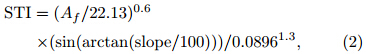
The modified RUSLE model is operated at an annualtimescale and covers the whole area of Alianello(7.34 km2). On this spatial scale, erosion processesare mostly controlled by soil type, l and use, and climatepatterns in relation to topography(Auzet et al., 2002).
On a side note, the RUSLE model only emphasizesrill and inter-rill erosion but does not considerthe sedimentation, which means the RUSLE resultsmerely show the potential erosion. To derive the Avalue in Eq.(1)for each pixel in our study area, eachfactor should be calculated by combining the correspondingmodel and the visual image interpretationtechniques. A summary of the soil erosion assessmentstrategies is given in Fig. 2.
 |
| Fig. 2. Strategies for the soil erosion assessment by combining visual image interpretation and RUSLE model technique. |
It should be emphasized here that the direct classificationof soil erosion from the interpreted geomorphologyis based on the erosion features in each geomorphologicunit. These features include(but are notlimited to)badl and s, dissected areas with gullies, and sheet or rill erosions. Three classes are given for thesoil erosion on the basis of the loss estimations fromthe modified RUSLE model: low, moderate, and high.These classes are interpreted according to differencesin soil tone and texture.
Finally, we perform a statistical validation of themodel(error matrix)through arranging the obtainedlinear channel volumes into three classes, allowingtheir comparison with modeled erosion classes usingthe adapted RUSLE.4. Results and discussion4.1 Geomorphologic characteristics
Based on the visual image interpretation fromGoogle image acquired by IKONOS(see Fig. 1 caption)in 2006, we obtain the geomorphic map and l and cover map(due to the limitation of space, the mapsare omitted here). The geomorphology over the studyarea of Alianello is generally hilly. Clearly, we canrecognize badl and s with erosion in process from thegeomorphic map. It is noticeable that the northernAlianello is on the moderately steep slopes with moderatelysevere badl and s development. In these hillyareas, one distinctive morphological environment canbe identified: bacK slopes and valleys covered by forest and tree plantation and the face slopes mostly byshrubs and grass. In the middle part of the study area, longitudinal highl and s with steep highly eroded faceslopes(associated with badl and development)consistof biancane and macro pediment, while in the backslopes, the area is on moderate steep slopes and coveredby mixed shrubs and grass. Towards the south, the hilly badl and s are continuing with different kindsof slopes, including steep eroded face slopes and agriculturefields of grassl and s in the bacK slopes. To thesoutheast, sharp hilly badl and s with calanchi show up, and it is possible that the erosion process of rills and gullies occurs.4.2 Factor map
The following subsections discuss factor estimationsfor use in the RUSLE model of this study.4.2.1 Rain erosivity
The R factor in the RUSLE model can be representedin the form of rain erosivity, which indicates thedriving force of sheet and rill erosion by rainfall and runoff. We worK out the R values from in-situ rainfallamount and intensity observations. In this study, thedatasets of daily rainfall amount are obtained from thesurrounding 40 weather stations, which are separatedabout 13 to 65 km apart. The data are first aggregatedinto annual rainfall amounts for the calculationof factor of rain erosivity in the RUSLE model.
The most straightforward approach is to deriverainfall value directly from the collocated elevationthrough a nonlinear regression. Unfortunately, the coefficientof determination between elevation and rainfallamount is as low as 0.36. The moving averageinterpolation method, therefore, is undertaken.
To simplify the procedure, several attempts havebeen made to directly derive the R factor based on theempirical relationship between R and rainfall amount(Renard and Freimund, 1994; Hu et al., 2000). Theequation developed by Renard and Freimund(1994)istaken for the estimation of R factor in this study asfollows:
where Pa denotes annual rainfall amount in mm.Based on Eq.(3), we derive the R factor map. Asshown in Fig. 3a, the R value increases gradually fromeast to west.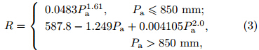
 |
| Fig. 3.(a)R factor map derived from rainfall measurements at the surrounding weather stations and (b)K factor map derived from ground surveyed measurements at the discrete stations. |
K factor, provided in point format, can be estimatedfrom ground surveyed measurements. We interpolatethe point value of K over continuous areausing the moving average method(Fig. 3b). It can befound that the K factor shows almost the same spatialpattern as the R value. This is possibly due to the factthat the K factor represents both susceptibility of soilto erosion and the amount and rate of runoff(Jones et al., 1996), which are closely associated with rainfall.4.2.3 STI index
As mentioned above, as a function of DEM and flow accumulation, STI is used to account for the effectof topography. Regarding how water and massfluxes are considered for the mass balance for eachpixel, a simple explanation was given by Burrough and McDonnell(1998). Flow accumulation, depending onthe drainage pattern of a terrain, quantifies how muchwater flows through each point of the terrain if waternaturally drains into outlets.
To estimate flow accumulation for every cell in agrid-based DEM, the flow direction is required to becalculated, which determines the natural drainage directionfor every cell of a terrain. Based on the flow directionresults, the flow accumulation function countsthe total number of pixels that will flow into outlets.Afterwards, flow accumulation is used in the computationof STI, which is in turn applied to model soilerosion through RUSLE.4.2.4 C and P factors
To represent better the effect of l and use and erosionconservation practice, RUSLE relies on C factorto consider the effect of cropping and management, while on P factor for support practices(Renard et al., 1997). Both C and P factors are related to the l and use identified by l and cover types.
To estimate C factor, NDVI should be first derivedfrom satellite images. Attempts have been madeto explore the relationship between C and NDVI, includingthe linear equation of Van der Knijff et al.(1999). Accounting for the limitation of a linear modelunder certain circumstances, we employ the followingequation to estimate C factor, which is strongly associatedwith l and cover.

The NDVI map from ASTER with 15-m resolution and the C factor map are given in Fig. 4a, withmost NDVI values between 0.16 and 0.64, whereas Cgenerally is less than 0.1.
 |
| Fig. 4.(a)NDVI map from ASTER acquired in 2006 and (b)C factor map based on NDVI. |
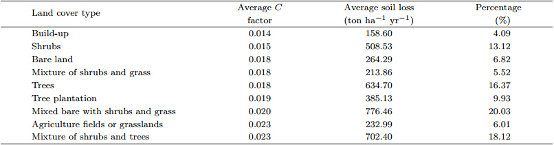
Through further statistical analyses, we find thatthe area covered by agriculture fields or grassl and s and mixture of shrubs and trees have the maximumC value(0.023)(Table 1).
Because not enough field observations have beentaken for l and cover type and l and use over the studyarea of Alianello, different P values corresponding tovarious l and cover types have been taken from the resultsfrom Jung et al.(2004)for use in the RUSLEmodel.4.3 Soil loss estimation
The soil loss values over the Alianello area arecalculated using Eq.(1). Figure 5 depicts the spatialpattern of soil loss. Three qualitative categories havebeen chosen for the output soil erosion classes: low, moderate, and high soil erosion susceptibility. FromFig. 5, it can be seen that the total annual soil lossin this region is less than 1400 ton ha−1 yr−1, exceptfor some spikes with extremely high value of 7000 tonha−1 yr−1 in the valleys with steep slopes.
 |
| Fig. 5. Annual total soil loss over Alianello in 2006 from the modified RUSLE model. |
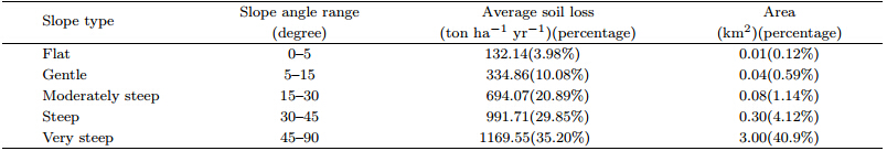
Table 2 shows that the very steep slope leads tothe risK of soil erosion, resulting in loss of 1169.55 tonha−1 yr−1(35.20%), while flat slope is the least susceptibleto soil erosion. Furthermore, it can be seenclearly from Table 2 that the steeper the slope, themore the soil loss. This holds true when no other factorslike conservative practice takes effect.
 |
As for the l and cover type(with respect to visualimage interpretation), it is more complicated. Table 1 shows that “mixed bare with shrubs and grass” isthe most susceptible(776.46 ton ha−1 yr−1)to soilerosion in this region, followed by “mixture of shrubs and trees”. Meanwhile, the type of “build-up” is themost resistant to soil erosion, but bare l and results ina soil loss as low as 264.29 ton ha−1 yr−1, which canbe attributed to the soil resistance to erosion or thegentle slope in these areas. To assess the accuracy ofthe produced table, validation with independent datais required, which can be obtained from field measurements, surveys, and high-resolution imagery. Unfortunately, the ground survey data are very limited inthis study and this should be further investigated inthe future.
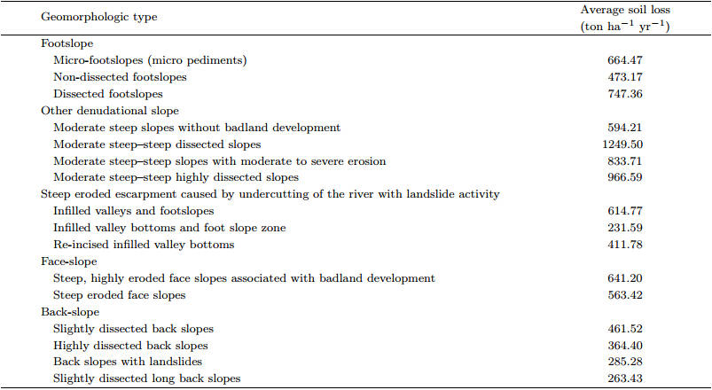
Regarding the vulnerability of geomorphologictype to soil erosion given in Table 3, the type of moderatesteep slope ranks the first, followed by foot slope, and bacK slope is the least vulnerable to erosion.
Although the model can yield quantitative valuesof soil erosion, the impact of individual factors such asP, K, l and cover, and topographic features(take STIhere for example)can only be explained in a qualitativesense(De Jong and Riezebos, 1997).
To assess where the future soil erosion will moreprobably occur in this study area, we calculate the averageannual soil loss mainly in terms of topographiccharacteristics of slope type, l and cover, and geomorphologictype, respectively. Based on the soil loss, thesusceptibility can be deduced accordingly.
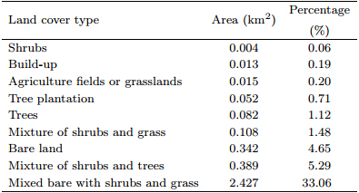
High erosion susceptibility areas indicate the highsoil erosion loss areas, as demonstrated in Fig. 5.Although there are actually several possibilities in extractingthem, the identified high erosion areas havebeen directly extracted from the erosion loss mapsaccording to the scheme described in detail in Section3.2. Namely, the erosion is classified as low(<1000 ton ha−1 yr−1), moderate(1000–5000 ton ha−1 yr−1), and high(5000–15000 ton ha−1 yr−1). Thehigh erosion susceptible area constitutes about 46.8%of the whole area and when classified by l and covertype, 33%(2.427 km2)is “mixed bare with shrubs and grass”, followed by 5.29%(0.389 km2)of “mixture ofshrubs and trees”, with “shrubs” having the lowestpercentage of 0.06%. Table 4 shows the percentagefor each l and cover type in detail.
 |
In terms of slope type, Fig. 6a shows that verysteep slope type accounts for a total of 40.90% of thestudy area belonging to the class of high susceptibility, whereas flat slope area only accounts for 0.12%, indicating the flat topography has a very limited effecton the erosion hazard. The details of percentage foreach slope class are given in Table 2.
 |
| Fig. 6. Soil erosion susceptibility classifications over the Alianello area in 2006 from(a)modified RUSLE model and (b)visual image interpretation. |
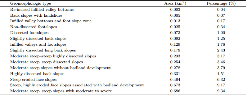
As far as the geomorphologic types are concerned, Table 5 shows that the type of “moderate steep–steepslopes with moderate to severe erosion” is most susceptibleto high soil erosion, which comprises about0.686 km2(9.34%). In contrast, the least area locatedin the high erosion area is the type of “re-incised infilledvalley bottoms” with 0.003 km2(0.04%).
 |
The validation of the erosion susceptibility fromthe adapted RUSLE model is of great importance forthis study. As Vrieling et al.(2006) and Kheir etal.(2006)described, validation can be accomplishedthrough ground truth survey and confusion matrix.However, there are always difficulties in erosion validationusing ground truth survey especially at locationswith complex terrain and private l and s where accessibilityis quite limited.
A quantitative validation of soil erosion by meansof field measurements is still a great challenge. As weknow, rills and gullies are the most distinct signs oferosion in the study area, whereby the visual interpretationfrom high resolution aerial photos to someextent can be thought as an alternative to validate themodel result.
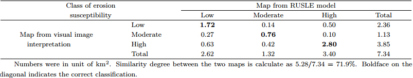
The quantitative erosion loss computation fromthe modified RUSLE model is carried out, wherebythe erosion susceptibility class map(Fig. 6a)is derivedbased on classification scheme described in Section3.2. Considering the unavailability of groundbasedmeasurements, the visually interpreted erosionresults from remotely sensed satellite images acquiredin 2006 are shown in Fig. 6b, as a means of validationagainst model results. The soil erosion susceptibilitymap(Fig. 6a)from the modified RUSLE model comprisesthe same classes(low, moderate, and high)asthose from visual image interpretation(Fig. 6b). Thehigh erosion class covers about 45% of the study areaon the erosion map from the adapted RUSLE modelbut increases to an area of 56% in the map from visualinterpretation. The increase of area in the mapshown in Fig. 6b is equivalent to 0.734 km2(10%).The comparison(in km2)of classes in the two mapsin Fig. 6 permits assessment of the effect of adaptedRUSLE model on erosion mapping(Table 6)in somedegree. In this contingency table, the sum of areasto which the classes of Figs. 6a and 6b correspondstrictly(km2; in boldface on the diagonal of the table)are divided by the total area of the study region(km2). Table 6 shows a similarity degree between thetwo maps of 71.9%, reflecting the major effect playedby the adapted RUSLE model in mapping the soil erosionin this study area.
According to Fig. 6, there are some differencesbetween the two erosion classification maps. Figure 6b shows that most of the area is hazard-prone tohigh erosion while Fig. 6a seems to show more details.Furthermore, the cross operation shows that there isalso a little difference between the erosion modeled and the image interpreted maps. The difference canbe caused by errors in image interpretation, lacK offield work, and the subjective characteristics of the inventorymap. Also, the soil factor used in the erosionmodel was produced by inadequate soil data, whichmay cause errors in the computation. The C and Pfactors were not rather accurate because the exact l and cover type and l and use practices must be studied foreach geomorphologic unit. All of these can contributeto the difference between the two erosion maps.5. Summary
In this paper, we employ the visual image interpretationtechnique from combination of stereoaerial photograph and satellite images to derive thegeomorphologic characteristics and l and cover overAlianello of southern Italy in 2006. Furthermore, theempirical model RUSLE for assessing soil erosion isused to investigate the soil erosion in this area. TheRUSLE model is a quantitative erosion model thathas fixed input parameters, which can be adapted tofit with available data accounting for locally importantprocesses and factors. We applied STI insteadof the combination of L and S to calculate the soilerosion. Apart from this, the soil erosion map is producedfrom visual image interpretation as a way ofvalidation against the RUSLE model output. The resultsshow that the similarity degree between the twoerosion maps from different methods amounts up to71.9%, indicating that the adapted model is a usefultool for assessing spatial variations in erosion patternsfor the study area where the terrain is quite rugged.
The estimation of soil loss using the modifiedRUSLE model has a large variance, ranging from 10to 7000 ton−1 ha−1 yr−1. Furthermore, it is observedthat the soil loss is closely associated with the degreeof terrain slopes. Besides, other factors such as l and cover influence the soil loss greatly as well.
On the basis of the maps produced from theadapted RUSLE model, it has become possible to assessthe spatial patterns in soil erosion and to identifyhigh erosion areas. Above all, the model could begood at prediction of the soil erosion. The modelederosion classification gives a quite realistic erosion predictionin comparison to the image interpreted erosionclassification. Also, the susceptibility and loss mappingreported in this paper can be adapted to othercountries which need an erosion assessment for theidentification of high erosion areas and priority actionareas.
Acknowledgments. The authors wish to thankDr. C. J. Cees van Westen and Doctor and us N.C. Kingma with International Institute for Geo-Information Science and Earth Observation(ITC), University of Twente, the Netherl and s for their kindsuggestions and comments on the susceptibility assessment.This worK was mainly finished at ITC, theNetherl and s.
| [1] | Auzet, A. V., J. Poesen, and C. Valentin, 2002: Soil patterns as a key controlling factor of soil erosion by water. Catena, 46, 85–87. |
| [2] | Basso, F., E. Bove, M. Del Prete, et al., 1996: The Agri Basin, Basilicata, Italy. Atlas of Mediterranean Environments in Europe: The Desertification Context. John Wiley and Sons, Inc., London, 144–149. |
| [3] | Burrough, P. A., and R. A. McDonnell, 1998: Principles of Geographic Information Systems. Oxford University Press, New York, 356 pp. |
| [4] | De Jong, S. M., and H. T. Riezebos, 1997: SEMMED: A distributed approach to soil erosion modelling. The 16th EARSel Symposium, Malta, 20–23 May 1996, 199–204. |
| [5] | Grimm, M., R. J. A. Jones, and L. Montanarella, 2003: Soil Erosion Risk in Italy: A Revised USLE Approach. European Soil Bureau Research Report No. 11, EUR 20677 EN. Office for Official Publications of the European Communities, Luxembourg, 26. |
| [6] | Hu, Q., C. J. Gantzer, P. K. Jung, et al., 2000: Rainfall erosivity in the Republic of Korea. J. Soil Water Conserv., 55(2), 115–120. |
| [7] | Jung, H. C., S. W. Jeon, and D. K. Lee, 2004: Development of soil water erosion module using GIS and RUSLE. The 9th Asia-Pacific Integrated Model (AIM) International Workshop, March 12–13, Tsukuba, Japan, 321–327. |
| [8] | Jones, D. S., D. G. Kowalski, and R. B. Shaw, 1996. Calculating revised universal soil loss equation (RUSLE) estimates on department of defense lands: A review of RUSLE factors and US army land condition-trend analysis (LCTA) data gaps. Center for Ecological Management of Military Lands, Department of Forest Science, Colorado State University, Fort Collins, Colorado, 1–9. |
| [8] | Kheir, R. B., O. Cerdan, and C. Abdallah, 2006: Regional soil erosion risk mapping in Lebanon. Geomorphology, 82, 347–359. |
| [9] | King, C., and G. Delpont, 1993: Spatial assessment of erosion: Contribution of remote sensing, a review. Remote Sens. Rev., 7, 223–232. |
| [10] | Lane, L. J., E. D. Shirley, and V. P. Singh, 1988: Modeling erosion on hillslopes. Modeling Geomorphological Systems. M. G. Anderson, Ed. New York City, John Wiley, Publ., 287–308. |
| [11] | Merritt, W. S., R. A. Letcher, and A. J. Jakeman, 2003: A review of erosion and sediment transport models. Environ. Model Software, 18(8–9), 761–799. doi: 10.1016/S1364-8152(03)00078-1. |
| [12] | Moore, I. D., P. E. Gessler, G. A. Nielsen, et al., 1993: Soil attribute prediction using terrain analysis. Soil Sci. Soc. Amer. J., 57(2), 443–452. |
| [13] | Morgan, R. P. C., 1995: Soil Erosion and Conservation. Longman Group Limited: Essex, UK, 298 pp. |
| [14] | Oldeman, L. R., V. W. P. Van Engelen, and J. H. M. Pulles, 1990: The extent of human induced soil degradation. Annex 5 of World Man of the Status of Human-Induced Soil Degradation: An Explanatory Note (2nd edition). Oldeman R. L., R. T. A. Hakkeling, and W. G. Sombroek , Eds., International Soil Reference and Information Center, Wageningen, 36. |
| [15] | Oliver, S., 1993: 20th-century urban landslides in the Basilicata region of Italy. Environ. Manage, 17(4), 433–444. |
| [16] | Pelletier, R. E., 1985: Evaluating nonpoint pollution using remotely sensed data in soil erosion models. J. Soil Water Conserv., 40(4), 332–335. |
| [17] | Renard, K. G., and J. R. Freimund, 1994: Using monthly precipitation data to estimate the R-factor in the revised USLE. J. Hydrol., 157(1–4), 287–306. |
| [18] | —–, G. R. Foster, G. A. Weesies, et al., 1997: Predicting soil erosion by water: a guide to conservation planning with the Revised Universal Soil Loss Equation. Agricultural Handbook, Vol. 703. U.S. Department of Agriculture, 404. |
| [19] | Servenay, A., and C. Prat, 2003: Erosion extension of indurated volcanic soils of Mexico by aerial photographs and remote sensing analysis. Geoderma, 117(3–4), 367–375. |
| [20] | Smith, S. J., J. R. Williams, R. G. Menzel, et al., 1984: Prediction of sediment yield from Southern Plains grasslands with the Modified Universal Soil Loss Equation. J. Range Manage., 37(4), 295–297. |
| [21] | UNESCO-FAO, 1963: Ecology of the Mediterranean zone. Bioclimatic Map of the Mediterranean Zone (Arid Zone Research XXI–5 maps with explanatory notes), Paris, 56. |
| [22] | Van der Knijff, J. M., R. J. A. Jones, and L. Montanarella, 1999: Soil erosion risk assessment in Italy. EUR 19044EN. European Soil Bureau. Office for Official Publications of the European Communities, Luxembourg, 52. |
| [23] | —–, —–, and —–, 2002: Soil erosion risk assessment in Italy. Proceedings of the Third International Congress Man and Soil at the Third Millennium. Rubio, J. L., Morgan, R. P. C., Asins, S., and V. Andreu, Eds. Geoforma Ediciones, Logrono, Spain, 903–1913. |
| [24] | Vrieling, A., 2006: Satellite remote sensing for water erosion assessment: A review. Catena, 65, 2–18. |
| [25] | —–, G. Sterk, and O. Vigiak, 2006: Spatial evaluation of soil erosion risk in the West Usambara Mountains, Tanzania. Land Degrad. Dev., 17, 301–319. |
| [26] | Wischmeier, W. H., and D. D. Smith, 1978: Predicting rainfall-erosion losses: A guide to conservation planning. Agricultural Handbook, Vol. 537. U.S. Department of Agriculture, 1–537. |