 2012, Vol. 26
The Chinese Meteorological Society
Article Information
- Wang Xiaoying, Song Lianchun, and Cao Yunchang. 2012.
- Analysis of the Weighted Mean Temperature of China Based on Sounding and ECMWF Reanalysis Data
- J. Meteor. Res., 26(5): 642-652
- http://dx.doi.org/10.1007/s13351-012-0508-2
-
Article History
- Received August 31, 2011
- in final form March 21, 2012


2 National Climate Center, China Meteorological Administration, Beijing 100081;
3 Meteorological Observation Center, China Meteorological Administration, Beijing 100081
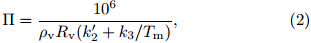
Water vapor is an active composition of the atmosphere, with extremely uneven distributions and largetemporal and spatial variations in the atmosphere.The phase change of water vapor is directly relatedto precipitation and plays an important role in theatmosphere energy transfer, weather development, radiationbudget of the earth-atmosphere system, and global climate change(Bevis et al., 1992; Rocken et al., 1995; Bi et al., 2006; Falconer et al., 2009; Perler et al., 2011). Low temporal and spatial resolutions of routineatmosphere observations restrict our knowledge on thespatiotemporal variation features of water vapor. As aresult, it leads to low precision of the initial humidityfield in numerical weather prediction(NWP)modelsas well as low accuracy of NWP results(Gutman et al., 2004; Song, 2004; Cao et al., 2005, 2006; Bastin et al., 2007). Ground-based GPS technology provides a newmean for atmospheric water vapor observation, whichcan be made all the time under all weather conditionsat high precision. It supplements the traditional atmosphereobservation methods(Song, 2004; Lutz, 2009).When using path wet delay(PWD)to obtain precipitablewater vapor(PWV)in ground-based GPStechnology, there are three important computation formulasas follows.
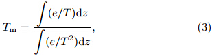
where Π is conversion coefficient, ρv is density of liquidwater equal to 1.0 g cm−3, Rv is gas constant forwater vapor equal to 0.4613 J g−1 K−1, and k’2 and k3are test constants of atmosphere refractive index equalto k’2=22.1±2.2 K hPa−1 and k3=(3.739±0.012)×105K2 hPa−1. As indicated by Eq.(3), Tm is the averagetemperature of the atmosphere weighted by the watervapor pressure, called the weighted mean temperature.
To evaluate the impact of Tm on the PWV, thefirst-order partial derivative is derived as follows:
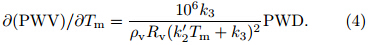
Typical values of zenith path hydrostatic delay(PHD)are 2.30 m and 0.00–0.40 m for PWD(Walpersdorf et al., 2001). Assuming the variables of PWD and Tm are constants, substitute the extreme values(e.g., PWD = 400 mm, Tm = 285 K)of all parameters intoEq.(4), the result is as follows:

Equation(5)shows that the Tm error of 1 K cancause a PWV error of 0.2243 mm in the case of a PWDvalue of 400 mm and Tm of 285 K. Therefore, accuratecalculation of Tm is important. In ground-based GPStechnology, there are several ways to acquire Tm:(1)considering Tm as a constant;(2)computing Tm byuse of a numerical integration method based on Eq.(3)using radiosonde data or numeral prediction products;(3)computing Tm from Ts(Ts denotes surfacetemperature)based on specific local Tm-Ts regressionmodels. In the above methods, considering Tm as aconstant may lead to low precision of Tm and PWV;the numerical integration method has the highest precision and Tm thus derived is often taken as the “true”observation, but it is difficult to apply this method toreal-time acquisition of Tm since the radiosonde dataor numeral prediction products are not available in thereal-time mode. Computing Tm from Ts based on theTm-Ts regression models is simple and easy with acceptableprecision in the current ground-based GPStechnology.
Most studies use statistical regression models toobtain Tm. Bevis et al.(1992)made an analysisof 8718 radiosonde profiles spanning approximatelya 2-yr interval for the stations in the United Stateswith the latitude range of 27°–65°N and a heightrange of 0–1.6 km, and yielded a linear regressionTm=70.2+0.72Ts. The RMS deviation from this regressionis 4.74 K, which is a relative error of less than2%. The Bevis regression model has been applied tomany studies of Tm in China(Li et al., 1999; Liu et al., 2006; Yue et al., 2008; Li et al., 2009; Yu and Liu, 2009; Wang et al., 2011a, b). However, it is found thatthe errors of the Bevis empirical model distribute unevenlyin China and are generally more than 4 K withthe extreme value of 8 K in some areas(Yu et al., 2011). The impact of the Bevis empirical model errorson the PWV can reach the millimeter level underan extreme weather condition with rich water vapor.
Previous studies focused on the setup of local Tm-Ts regression models for a specific region based onsounding data(Li et al., 1999; Liu et al., 2006; Yue et al., 2008; Li et al., 2009; Wang et al., 2011a). Yu and Liu(2009) and Yu et al.(2011)discussed the errorstatistics of the Bevis model over China and gave thedependence of the errors on the elevation of station.Wang et al.(2011b)investigated the correlation of thecoefficients a and b of the local Tm model with longitude, latitude, and station elevation. Nonetheless, some aspects such as the spatiotemporal distributioncharacteristics of Tm and the associated retrieval errorcomparison between the Bevis model and local modelsover entire China are rarely researched. Yu and Liu(2009)presented a method adding a correction relevantto elevation in the Bevis model to obtain Tm overareas without historical sounding data.
Reanalysis of multi-decadal series of past observationshas been widely utilized for the studies of atmospheric and oceanic processes and predictability.Since reanalysis data are produced using sophisticated and advanced data assimilation systems developed forNWP, they are more suitable than operational analysisfor use in studies of long-term variability of climate.Reanalysis products are used increasingly in manyfields that require an observational record of the stateof either the atmosphere or its underlying l and and ocean surfaces. So far, ECMWF has produced threereanalysis products including ERA-15, ERA-40, and ERA-interim, among which ERA-interim is a globalreanalysis of the data-rich period since 1989. TheERA-interim data assimilation system uses a 2006release of the Integrated Forecasting System(IFSCy31r2), which contains many improvements in boththe forecasting model and the analysis methodology, compared to those for ERA-40. The ERAinterimreanalysis was put into operation in March2009, and has been running in near real-time tosupport climate monitoring(http://www.ecmwf.int/research/era/do/get/Reanalysis−ECMWF, retrievedon 19 December 2011).
This study adopts the numerical integrationmethod and the sounding data of 87 internationalexchange sounding stations in China to obtain thespatiotemporal distribution characteristics of Tm overChina. Meanwhile, we compare the results of Tm calculatedfrom the Bevis model with those from thelocal regression models based on historical soundingdata, and then evaluate the performance of the Bevismodel and the local Tm-Ts regression models. Whensetting up regression models for areas without soundingdata, the Kriging spatial interpolation method isused to obtain the coefficients of the local Tm-Ts regressionmodels and the results are assessed in comparisonwith the numerical method results using the soundingdata. In addition, the Tm-Ts regression model resultsbased on the ERA-interim reanalysis product are alsocompared with those based on the sounding data ofBeijing and Hong Kong(HK), and the results indicatethat the ERA-interim reanalysis provide anotherdata source for local Tm calculation in areas withoutsounding data.2. Data and method
In this paper, we use local Tm-Ts regression modelsbased on sounding data or the ERA-interim reanalysisproduct to derive Tm, and use the “true” observationcalculated from the sounding data with thenumerical integration formula to validate the regressionresults. The data of 87 international soundingstations in China for 2003–2010 are downloaded fromthe University of Wyoming website http://weather.uwyo.edu/upperair/sounding.html(retrieved on 19December 2011). The ERA-interim data are downloadedfrom http://data-portal.ecmwf.int/data/d/interim−daily(retrieved on 19 December 2011).
The numerical integration method is a discretionform of Eq.(3) and is described below. Tm can be retrievedfrom both sounding data and reanalysis productsas follows(Li et al., 1999; Liu et al., 2006; Yue et al., 2008; Li et al., 2009; Yu and Liu, 2009; Wang et al., 2011a, b).
where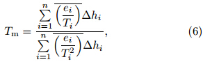
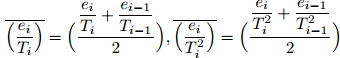 , Δhi is the thickness of ith layer atmosphere, ei and Ti are upper bound water vapor pressure and temperatureof ith layer atmosphere respectively, and ei−1 and Ti−1 are lower bound water vapor pressure and temperature of ith layer atmosphere respectively.For sounding data, the water vapor pressure isequal to saturated vapor pressure of dew point temperature.
For reanalysis product ERA-interim, the temperature, geopotential height(H), and relative humidity(RH)fields have a resolution of 1.5° latitude ×1.5°longitude and 37 vertical levels. The surface temperature(Ts) and surface dew point temperature fields atthe same horizontal resolution are also used. All variablesare available 4 times daily at 0000, 0600, 1200, and 1800 UTC. The water vapor pressure(e)is obtainedfrom RH and saturation water vapor pressure(E)as follows:
When Eq.(6)is used to calculate Tm, all data at thelevels below the station’s geopotential height value arediscarded. The surface water vapor pressure is calculatedfrom the surface dew point temperature.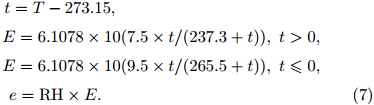
When comparing the Tm values obtained fromsounding with that obtained from ERA-interim basedon Eq.(6), interpolations are conducted as follows. Inthe vertical direction, the level at which the station islocated is determined according to the station’s actualgeopotential height. Linear interpolation is used to obtainthe surface temperature of the station based onthe reanalysis data of two adjacent vertical grids, and exponential interpolation is used to obtain its watervapor pressure. In the horizontal direction, the temperature and water vapor pressure at each level abovethe station are obtained using bi-linear interpolationbased on data of the four adjacent grids at the samelevel.
The Tm-Ts regression model is obtained usingMatlab based on historical Tm and Ts sample pairsas follows. First, Tm is calculated by Eq.(6)twicea day for sounding data and four times a day forERA-interim reanalysis product. Note that Ts canbe directly obtained from the sounding data or ERAinterimreanalysis product. Then, the Tm-Ts regressionmodel based on the total samples in a certain periodof time can be set up with the Matlab software.For example, during a one-year period, there are about730 samples for sounding data and 1460 samples forERA-interim reanalysis product. The precision of theTm-Ts regression model is evaluated by comparing Tmcalculated by Eq.(6)with Tm calculated by the Tm-Tsregression model.3. Regression of Tm at HK by seasons based on the sounding data
Based on the sounding data of HK(WMO stationID 45004)in 2005, Tm of this station was calculatedby Eq.(6). Figure 1 shows the Tm annual change in2005. Tm varies significantly by season between 275 and 295 K with the highest value in summer and lowestin winter. This gives us a rough idea of how Tmchanges with season. It also raises a question as toif it is better to establish seasonal regression modelsaccording to seasonal sounding data rather than toobtain general/annual regression models according toconsecutive multi-year sounding data time series, i.e., if seasonality of the regression should be considered and could be used to facilitate the regression accuracy?
 |
| Fig. 1. Annual change of Tm obtained by using the numerical integration method and the 0000 and 1200 UTC sounding data of HK in 2005. |
In this section, the precision of the annual and seasonal Tm-Ts regression models for the HK stationbased on the sounding data are evaluated. There are59 missing records for a total of 4325 valid times forthe period 2003–2008 for HK sounding station. TheHK−annual Tm-Ts model in Table 1 is set up basedon all the sounding data from 2003 to 2008. We classifythe total sounding data of 4325 entries from 2003to 2008 by season, and about 1080(Tm and Ts)samplesare obtained for every season. Based on that, four seasonal Tm-Ts empirical models are set up, calledHK−season(spring, summer, autumn, and winter), asshown in Table 1. Table 1 indicates that the a and bcoefficients of spring and autumn models are close tothat of the annual model, while the a and b coefficientsof summer and winter models differ largely from thatof the annual model.
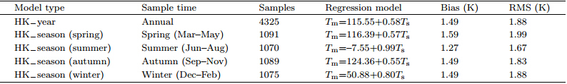
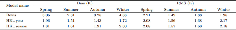
We use the sounding data of HK station in 2009to validate the local seasonal Tm-Ts empirical models.The values of Tm in 2009 are calculated using Eq.(6) and taken as real values. With regard to the seasonalregression models in Table 1, there are a total of 730(Tm and Ts)samples in 2009 with averagely 185 samplesin every season. The model values of Tm for thefour seasons in 2009 are calculated from the seasonalTm-Ts empirical models, respectively, and their statisticresults are shown in Table 2. Although the a and bcoefficients of summer and winter models differ largelyfrom that of the annual model, there is almost no differencewhen replacing any of the seasonal models withthe annual one to calculate Tm. On the contrary, theBevis model has a larger bias than local seasonal modelsbut almost the same RMS.
 |
Why do the a and b coefficients of the summer and winter models differ largely from that of the annualmodel, but the Tm values differ little from thatcalculated from their linear combination? The lineartrends of Tm from the four seasonal models and theannual model are shown in Fig. 2. The summer temperaturein HK varies from 299.15 to 306.15 K(yellowvertical range)with the mean value of 301.15 K, whilethe winter temperature in HK varies from 287.15 to293.15 K(lavender vertical range)with the mean valueof 290.15 K. Figure 2 shows that the trend line of Tmfrom the summer model is very close to that from theannual model within the temperature range of 299.15–306.15 K, so is that with the winter model and annualmodel for the temperature range of 287.15–293.15 K.Thus, Tm calculated from the specific seasonal model and annual model is almost the same.
 |
| Fig. 2. Trend lines of the seasonal and annual regression models for HK. |
The average monthly Tm in January, April, July, and October is calculated based on the sounding datafrom 2003 to 2009 by Eq.(6)to reveal the spatial and temporal distribution characteristics of Tm overChina. The results are shown in Fig. 3.
 |
| Fig. 3. Spatial distributions of the average monthly Tm(K)calculated by using the sounding data and Eq.(6)overChina in(a)January, (b)April, (c)July, and (d)October. |
Figure 3 shows that the average monthly Tm oversoutheastern China is the highest throughout the year, whereas it is the lowest over northeastern China inJanuary and over the Qinghai-Tibetan Plateau in July.
The general characteristics of spatiotemporal distributionsof the average monthly surface temperatureTs in China are consistent with Tm. The correlationcoefficient between Tm and Ts is 0.848(Wang et al., 2011b), which shows the feasibility of estimating Tmby Ts.
Previous studies(e.g., Li et al., 1999; Liu et al., 2006; Yue et al., 2008; Li et al., 2009; Yu and Liu, 2009; Wang et al., 2011a, b)never investigated theoverall spatiotemporal distribution of Tm over China.Figure 3 shows that the Tm distributions may havesomething to do with the climate pattern, populationdensity, and topography. Southeastern China is underthe influence of the subtropical monsoon climate withhigh population density, and Tm is relatively high inthis region throughout the year. Northeastern Chinais dominated by the temperate monsoon climate, and Tm is comparatively low all the year except in summer.Tm over the Qinghai-Tibetan Plateau is significantlylow compared with other areas in summer because ofits unique topography.4.2 Tm distribution by the regression method based on the sounding data
There are 120 sounding stations in China, amongwhich 87 are international exchange stations. Thedata of the 87 stations from 2009 to 2010 are examined.We use the radiosonde data of 2009 to obtain thelocal Tm-Ts regression model for each station, then usethe sounding data of 2010 to evaluate the local model and compare with the Bevis model.
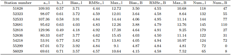
The results shown in Table 3 and Fig. 4 revealthat not all the local Tm-Ts models are more precisethan the Bevis model; this is inconsistent with theconclusion of previous studies(Li et al., 1999; Liu et al., 2006; Yue et al., 2008; Li et al., 2009; Yu and Liu, 2009; Wang et al., 2011a, b). In Table 3, dTm meansthe difference between the real value of Tm in 2010 byEq.(6)using sounding data and the model value ofTm by the local Tm-Ts model or the Bevis model usingthe radiosonde data of 2009, where a−l is the a coefficientof the Tm-Ts model and same is for b_l. TheBias_l, RMSe_l, Max_l, and Num_l are respectivelythe mean bias, st and ard deviation, maximum valueof dTm, and the number of samples with dTm greaterthan five degrees based on the local model. Similarly, the Bias_B, RMSe_B, Max_B, and Num_B are thecorresponding statistical variables for the Bevis model.The number of samples is about 730 in 2010.
 |
| Fig. 4. Distribution of the number of samples with the Tm difference more than 5 K calculated from the Bevis model and the local Tm-Ts model based on the sounding data in China. |
The results indicate that there are 22 soundingstations for which the local Tm-Ts models are not betterthan the Bevis model. Table 3 only lists the statisticalinformation of 9 stations. Table 3 and Fig. 4show that the Bevis model is fit for areas of northeasternChina and the Qinghai-Tibetan Plateau while ithas a large deviation in southeastern and northwesternChina, where the local Tm-Ts model works better.5. Regression of Tm at two stations using the Kriging method based on the sounding data
The Kriging interpolation method provides an unbiasedoptimal estimation for regional variables in alimited area based on variation function spatial analysis.It takes into account the spatial correlation betweenthe data points and is suitable for interpolationof spatial data. Details for Kriging interpolation canbe seen in Zeng and Huang(2007).
The average distance of adjacent sounding stationsis about hundreds of kilometers. For southeastern and northwestern China, the local Tm-Ts modelsare difficult to set up due to the absence of soundingdata. The Kriging spatial interpolation methodis used to obtain the a and b coefficients of the localTm-Ts models for areas without sounding data. Thismethod is evaluated at two sounding stations, i.e., Pizhou(WMO station ID 57972) and Kuche(WMOstation ID 51644). Pizhou station locates in southeasternChina where a dense network of sounding stationsexists, whereas Kuche station locates in northwesternChina where there is a lack of sounding stations. Selectingthe two stations for test can validate if theKriging interpolation method is able to obtain localTm-Ts models for areas with both dense and coarsedistributions of sounding stations at acceptable precision.For areas such as southeastern and northwesternChina where the Bevis model fails to perform well, thelocal Tm-Ts models should be set up.
The evaluation for Pizhou station is conducted asfollows: 1)use the Kriging method to generate a and b isosurfaces based on the a and b coefficients of therest of the 86 sounding stations; 2)obtain the interpolatedvalues of the a and b coefficients for this station, and the Kriging Tm-Ts model for this station is thenobtained; 3)use the observed sounding data of 2010to derive a real local Tm-Ts model, compare with theKriging model derived in step 2, and calculate theirdifferences. The same process as described above isapplied to Kuzhe station. The results are shown inTable 4.
 |
In Table 4, a_k is the a coefficient of the Tm-Tsmodel based on the Kriging interpolation method and same holds for b_k. The Bias_k, RMSe_k, Max_k, and Num_k are respectively the mean bias, st and arddeviation, maximum value of dTm, and the numberof samples with dTm greater than five degreesbased on the Kriging method. The a_l, b_l, Bias_l, RMSe_l, Max_l, and Num_l are the same as inTable 3.
Table 4 shows that the Kriging spatial interpolationmethod is feasible in setting up the appropriatelocal Tm-Ts model for areas with no historical soundingdata such as southeastern and northwestern China, where the Bevis model performs not well.6. Evaluation of Tm at Beijing and HK calculated by the numerical and regression methods from two data sources6.1 Tm values calculated by the numerical method from both data sources
We used ERA-interim and sounding data of 2003for Beijing and 2007 for HK to derive Tm values byEq.(6). The results are shown in Table 5.
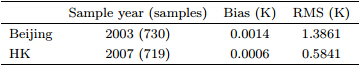 |
There are 1460 samples for the ERA-interim datain both 2003 and 2007, from which 730 samples matchthe time of the sounding data for 2003 and 719 samplesfor 2007. Table 5 shows that there is little differencebetween the Tm values calculated by Eq.(6)fromthese two different datasets.
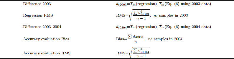
Statistical analysis in Table 5 is performed in thefollowing way:
Difference: di = Tm(ERA interim)− Tm(sounding);
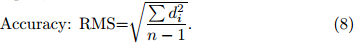
Systematic error: Bias= , where n is numberof samples;
Once the local Tm-Ts empirical formula has beenset up, Tm can be calculated by Ts with high precision, and it can then be used to obtain PWV using PWDin ground-based GPS. We set up a Tm-Ts empiricalformula using the ERA-interim data of 2003 for Beijing and 2007 for HK. The accuracy of this empiricalformula is evaluated by the ERA-interim data of 2004for Beijing and 2008 for HK. The statistical results arelisted in Table 6.
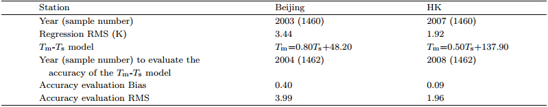 |
How the statistical analysis in Table 6 was performedis detailed in Table 7 for both Beijing and HK.
To further underst and the regressed Tm valuesfrom the ERA-interim data, the corresponding soundingdata were also processed. Comparisons of Tm bythe ERA-interim and sounding data are shown in Table 8. Table 8 shows that the local Tm-Ts empiricalmodel(Tm-Ts)EAR-interim based on the EAR-interimreanalysis data coincides well with that based on thesounding data.
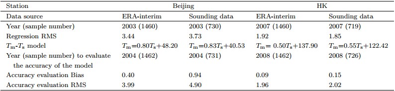 |
To sum up, the above comparisons demonstratea good agreement between ERA-interim reanalysisproduct and sounding data when calculating Tm basedon the numerical integration method and when settingup Tm-Ts regression models in Beijing and HK. This iseasy to underst and since radiosonde data are the key and main data source for the assimilation of reanalysisproducts. For areas with rich sounding data, the reanalysisproduct in general has good quality too. Itis also proved that the ECMWF reanalysis productERA-interim can be applied to the acquisition of Tmfor Beijing and HK areas.7. Conclusions
This paper first compares the difference betweenthe annual and seasonal Tm-Ts regression models forHK in detail and then examines the applicability of theBevis Tm-Ts regression model over China. For areaslack of historical sounding data, the Kriging interpolationmethod and the ECMWF reanalysis productERA-interim are used to set up local Tm-Ts models.We draw the following conclusions:
(1)The annual and seasonal Tm models have considerableaccuracy, Tm can be calculated precisely byannual Tm model for all seasons, and it is not necessaryto set up local seasonal Tm models for HK soundingstation.
(2)The Bevis model is fit for areas of northeasternChina and the Qinghai-Tibetan Plateau, butit produces a large deviation of Tm in southeastern and northwestern China, where the local Tm-Ts modelshould be set up.
(3)The Kriging spatial interpolation method canbe used to set up the local Tm-Ts model for areas withno historical sounding data such as southeastern and northwestern China, where the Bevis model performsnot well.
(4)Acquisition of the local Tm based on ERAinterimreanalysis data coincides well with that basedon the sounding data for Beijing and HK, which mightprovide a substitute available data source to set uplocal Tm-Ts models for areas lack of sounding data.
For areas lack of historical sounding data, theKriging interpolation method and the ECMWF reanalysisproduct ERA-interim were both employed toset up the local Tm-Ts model. The ECMWF reanalysisproduct has wide data coverage and long data spanon acceptable grid resolutions, whereas for the Krigingmethod in Section 5, there are only 120 soundingstations in China. Future research may focus on thevalidation of the ECMWF reanalysis product ERAinterimin setting up local Tm-Ts models in comparisonwith the Kriging method. If the result is encouraging, the ECMWF reanalysis product can be used to set upthe local Tm-Ts models on the grid scale. Meanwhile, the Kriging method may also be used to interpolatedthe a and b coefficients of the local Tm-Ts models formore homogeneously and rich distributed grids.
It should be pointed out that because the qualityof the reanalysis product strongly depends on thequality and richness of the sounding data, for areaswith no or few sounding data, the quality of the reanalysisproduct may not be good. It is difficult to saywhether the reanalysis product is fit for Tm calculationfor areas without sounding data. Nevertheless, it willbe the direction of further research about whether thereanalysis product might serve as an effective and richdata source for the acquisition and localization of Tmfor areas with no sounding data.
Acknowledgments. The ECMWF ERAinterimdata used in this study are provided by theECMWF, and sounding data are provided by the Universityof Wyoming.
| [1] | Bastin, S., C. Champollion, O. Bock, et al., 2007: Diurnal cycle of water vapor as documented by a dense GPS network in a coastal area during ESCOMPTE IOP2. Bull. Amer. Meteor. Soc., 46, 167–182. |
| [2] | Bevis, M., S. Businger, T. A. Herring, et al., 1992: GPS meteorology: Remote sensing of atmospheric water vapor using the global positioning system. J. Geophys. Res., 97(D14), 15787–15801. |
| [3] | Bi Yanmeng, Mao Jietai, Liu Xiaoyang, et al., 2006: Use ground-based GPS to sense slant path integrated water vapor. Chinese J. Geophys., 49(2), 335–342. |
| [4] | Cao Yunchang, Fang Zongyi, and Xia Qing, 2005: Preliminary analysis on the correlation between GPS sensed integrated water vapor and regional precipitation. J. Appl. Meteor. Sci., 16(1), 54–59. (in Chinese) |
| [5] | —–, Chen Yongqi, Li Binghua, et al., 2006: The method of using ground-based GPS to obtain atmospheric water vapor profile. Meteor. Sci. Tech., 34(3), 241–245. (in Chinese) |
| [6] | Gutman, S. I., S. R. Sahm, S. G. Benjamin, et al., 2004: Rapid retrieval and assimilation of ground based GPS precipitable water observations at the NOAA Forecast Systems Laboratory: Impact on weather forecasts. J. Meteor. Soc. Japan, 82, 351–360. |
| [7] | Falconer, R. H., D. Cobby, P. Smyth, et al., 2009: Pluvial flooding: New approaches in flood warning, mapping and risk management. J. Flood Risk Manage, 2, 198–208. |
| [8] | Li Guocui, Li Guoping, Du Chenghua, et al., 2009: Research on weighting mean temperature model during water vapor inversion using ground-based GPS in North China area. J. Nanjing Inst. Meteor., 32(1), 81–86. (in Chinese) |
| [9] | Li Jianguo, Mao Jietai, and Li Chengcai, 1999: The principle of using GPS to sense water vapour distribution and regression analysis on weighing mean temperature in eastern China. Acta Meteor. Sinica, 57(3), 283–292. (in Chinese) |
| [10] | Liu Xuchun, Wang Yanqiu, Zhang Zhenglu, et al., 2006: The comparison analysis on the obtaining method of weighting mean temperature when using groundbased GPS to sense atmospheric integrated water vapor. Journal of Beijing University of Civil Engineering and Architecture, 22(2), 38–40. (in Chinese) |
| [11] | Lutz, S., 2009: High-resolution GPS tomography in view of hydrological hazard assessment. PH. D. dissertation, ETH ZURICH, i-vi. |
| [12] | Perler, D., G. Alain, and H. Fabian, 2011: 4D GPS water vapor tomography: New parameterized approaches. J. Geodesy., 85(8), 539–550. |
| [13] | Rocken, C., van H. T., J. Johnson, et al., 1995: GPS/STORM-GPS sensing of atmospheric water vapor for meteorology. J. Atmos. Ocean. Technol., 12, 468–478. |
| [14] | Song Shuli, 2004: Monitor water vapor three-dimensional distribution using ground-based GPS network and its usage in meteorology. Ph. D. dissertation, Shanghai Astron. Obs., 1–14. (in Chinese) |
| [15] | Walpersdorf, A., E. Calais, J. Haase, et al., 2001: Atmospheric gradients estimated by GPS compared to a high resolution numerical weather prediction (NWP) model. Physics and Chemistry of the Earth, 26(3), 147–152. |
| [16] | Wang Xiaoying, Song Lianchun, Dai Ziqiang, et al., 2011a: Feature analysis of weighted mean temperature Tm in Hong Kong. Journal of Nanjing University of Information Science & Technology (Natural Science Edition), 1, 47–52. |
| [17] | —–, Dai Ziqiang, Cao Yunchang, et al., 2011b: Weighted mean temperature statistical analysis in groundbased GPS in China. Geomatics and Information Science of Wuhan University, 36(4), 412–416. (in Chinese) |
| [18] | Yu Shengjie and Liu Lintao, 2009: Verification and analysis on water vapor weighting mean temperature regression formula. Geomatics and Information Science of Wuhan University, 34(6), 741–744. (in Chinese) |
| [19] | —–, Wan Rong, and Fu Zhikang, 2011: Research on localization of weighted mean temperature in GPS water vapor sounding. Conference on New Data Usage in Heavy Rain Sounding. Hubei, 8–10 February, Institute of Heavy Rain, China Meteorological Administration, Wuhan, 15–20. (in Chinese) |
| [20] | Yue Yingchun, Chen Chunming, and Yu Yan, 2008: Research on the usage of GPS technology to sense atmospheric water vapor in the South Pole area. Sci. Survey Map., 33(5), 81–84. (in Chinese) |
| [21] | Zeng Huaien and Huang Shenxiang, 2007: Research on spatial data interpolation based on Kriging interpolation. Engineering of Surveying and Mapping, 16(5), 5–10. (in Chinese) |