 2012, Vol. 26
The Chinese Meteorological Society
Article Information
- Yang Chengyin, Lu Qifeng, and Zhang Peng. 2012.
- A Study on Height Reassignment for the AMV Products of the FY-2C Satellite
- J. Meteor. Res., 26(5): 614-628
- http://dx.doi.org/10.1007/s13351-012-0506-4
-
Article History
- Received September 15, 2011
- in final form April 17, 2012


2 National Satellite Meteorological Center, Beijing 100081;
3 Harbin Air Force Flight Academy, Harbin 150001
Satellite-derived atmospheric motion vectors(AMVs)play a significant role in a number of meteorologicalfields. In particular, the assimilation ofAMVs into forecast initialization conditions can resultin improvements in the forecast skill(Rohn et al., 2001; Zapotocny et al., 2008; Steinhoff, 2009). Heightassignment is the most crucial and challenging issue inthe computation of AMVs. Velden and Bedka(2008)noted that inaccurate height assignment was fundamentallyresponsible for 70% of the total errors inAMVs. Schmetz and Holmlund(1992), Nieman et al.(1993), and Borde and Oyama(2008)have all echoedthis conclusion in their respective work. Numerousstudies have been carried out to improve the accuracyof operational AMV height assignments, mainly employingeither geometric or physical methods.
The geometric method, initially by Hasler(1981), depends only on the basic geometrical relations amongcloud masses. This method generally assigns accurateheights, but is only applicable to areas where twosatellites overlap spatially and temporally. This dualsatelliterequirement makes the geometric methodsuitable for checking the validity of height assignments, but challenging for implementation in operationaluse. Despite this difficulty, some progress hasbeen made by jointly merging observations from twosatellites or by merging multi-angle observations froma single satellite(Diner et al., 1999).
The physical method, which is more widely employed, assigns height according to the correlations betweenobserved and simulated double-channel brightnesstemperatures. This method depends on the forecastsof atmospheric profiles and cloud top temperaturefrom numerical weather prediction(NWP)models, and is often called the double-channel method.The method accounts for the fact that infrared brightnesstemperatures can only be used to determine theheights of opaque clouds, and cannot be used to determinethe heights of semitransparent cirrus clouds. Thedouble-channel method was initially proposed by Szejwach(1982), who called it the water vapor interceptmethod. Szejwach(1982)improved the assignment ofcloud height considerably by jointly employing an infraredchannel(11.2 μm) and a water vapor channel(6.7 μm). This dual-channel approach is regarded asa classic principle in the search for methods of assigningheight to AMVs. Menzel et al.(1983)suggestedthat the CO2 channel could be used for this purpose, as it is semitransparent. This method requires additionalobservational instrumentation. Building on theunderst and ing of cloud height information within theinfrared and water vapor channels, Xu et al.(1997, 1998)improved the double-channel algorithm by processinghigh, middle, and low clouds separately. Thisapproach not only yielded a greater number of moreaccurate AMVs, but also enabled more accurate retrievalsof cloud top heights. The biases from NWPforecast profiles, which are used in the height assignmentalgorithm, degrade the accuracy of AMV heightassignments. AMVs derived from EUMETSAT(EuropeanMeteorological Satellite)using 61-layer NWPprofiles are partially responsible for forecast biasesover the Atlantic Ocean; these biases can be reducedsubstantially by using 91-layer NWP profiles for AMVheight assignment instead(personal communicationwith Dingmin Li, Met Office). Xue(2009)also demonstratedthe necessity of studying how the products ofChinese NWP models could be used to reduce sucherrors.
To this point, no favorable solution to the inaccuracyof height assignment has been put forward.This issue has become a major obstacle in the operationalapplication of AMVs(Li et al., 2009). A secondAMV intercomparison study with particular focuson height assignment was recommended by the WMOthrough CGMS-38 Action WGII 38.27(www.cgmsinfo.org/dl/CGMS-38−Report.pdf), with the broadaim of dynamically improving NWP forecasts throughthe assimilation of AMVs. This intercomparison wasjoined by the NOAA(National Oceanic and AtmosphericAdministration), ECMWF(European Centrefor Medium-Range Weather Forecasts), EUMETSAT, CMA(China Meteorological Administration), JMA(Japan Meteorological Agency), and others.
The NSMC(National Satellite MeteorologicalCenter)FY-2 AMV group is persistently working towardimproving the data-quality of AMVs derivedfrom FY-2, with special attention to height assignment.For example, using principles of fluid continuitywithin a certain range, Chen et al.(1999)setaccurate heights for some “inappropriate” winds byusing AMVs on other heights as a reference. This approachgreatly improved the quality of wind vectorsat low levels, particularly at 850 hPa. In 2011, theFY-2 AMV algorithm was improved in several technicalareas, including the replacement of the originalT213 forecast with a more accurate T639 forecast and the incorporation of a more accurate radiative transfermodel. These changes have resulted in improvementin AMV height assignment, as confirmed by analysisof error statistics at NSMC/CMA and FY-2E operationalmonitoring at the UK Met Office and ECMWF(personal communications with Jianmin Xu at NSMC, James Cotton at the UK Met Office, and Niels Bormannat ECMWF). The improvement was indeed observedwhen the diagnostic method proposed by Yanget al.(2012)was used; however, the diagnostic resultssuggest that there is still much to be done to improvethe data quality.
Yang et al.(2012)analyzed the bias distributioncharacteristics of derived AMVs from FY-2C satelliteto better underst and the main sources of uncertainty and bias. Their results indicated that the AMVs aretypically biased high and this bias shows features of aclimatic distribution. By introducing a simple prototypeheight reassignment model with the NCEP(National Centers for Environmental Prediction)reanalysisas a reference, the AMVs were reassigned to newheights. Comparison of satellite-derived AMVs withradiosonde data before and after the height reassignmentconfirmed that the biases were reduced and theclimatic distribution of the bias was largely eliminated.However, that study only put forward a proto-typeheight reassignment method, with little exploration ofthe rationale or technical details. This paper will discussthe reassignment methods in more detail so as tohelp the FY-2 AMV retrieval algorithm group betterunderst and height assignment biases and to furtherthe improvement of FY-2 AMV data quality. Threepossible schemes are presented, and then the NWPforecast fields are applied to height reassignment usingeach of these schemes. The feasibility of usingthese schemes to operational diagnosis of AMV biasesis also studied.2. Data and methodology2.1 Data
The AMVs used herein are cloud-derived windscomputed by the NSMC from the infrared channel(IR1) and water vapor channel(IR3)of the FY-2Cgeostationary meteorological satellite. The FY-2Csatellite was independently developed by China and put into operation on 1 June 2005 as the first suchsatellite in operation in the country. At present, theNSMC has used only the infrared and water vapor imagechannels in the calculation of AMVs1 . This paperemploys AMV data from September 2008. These dataare provided four times daily at a horizontal resolutionof 1°×1° over the area 50°S–50°N, 55°–155°E.
Other data used in this analysis include theNCEP/FNL(NCEP finalized analysis)gridded data, with a horizontal resolution of 1°×1° and a verticalresolution of 26 layers; radiosonde observations frominternational exchange stations; and the forecast fieldfrom a T511 mid-range numerical model, which has ahorizontal resolution of 1°×1° and a vertical resolutionof 17 layers.2.2 Calculation of consistency coefficient
According to the principle of continuity in fluidmovement, the velocities of neighboring fluid particlesare relevant and consistent in both speed and direction.This principle also holds for fluid movement atlarge scales. The closer the two particles are, the moreconsistent their velocities should be. AMVs assignedto incorrect heights can be entirely inconsistent withthe ambient wind fields at those heights. Based onthe principle of consistency, satellite-derived AMVsare compared with relatively reliable reference windfields in this paper. Incorrect heights are revised accordingto the results of these comparisons.
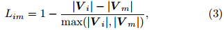
According to Wu(1993), the consistency coefficientbetween the AMV Vi at point i and the ambientwind vector V m at the neighboring point m canbe calculated as
where Dim is the consistency coefficient for wind direction and Lim is the consistency coefficient for windspeed. These two components can be described separately aswhere θim is the difference between the directions ofthe two wind vectors.

The general consistency between the AMV atpoint i and the ambient wind field within a radius Rof point i can be calculated by independently calculatingthe consistency coefficients between the AMV and each of the reference wind vectors that is at the sameheight and within that radius. The individual coefficientsare then weighted by the distances between thepoint i and the corresponding reference wind vectors.The weighting function with distance R is
where rim is the distance between points i and m. Theoverall consistency coefficient can then be computed asIn this way, the parameter ρi provides a quantitativemeasure of consistency.2.3 The height reassignment schemes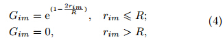
Each AMV is compared with reference wind fieldsat the same height and at other nearby heights, withthe assumption that the horizontal wind vector of theAMV is accurate. Three schemes for height reassignmentare designed as follows.
Scheme 1: Using the NCEP/FNL wind field as areference, the consistency coefficient between Vi and the reference wind vectors within a radius of 200 kmis calculated on each layer. A threshold ρo is defined(0.7 herein)for comparison with the consistency coefficientat the original assigned height of Vi. If theconsistency coefficient exceeds ρo, no adjustment isperformed. Otherwise, the height of the layer with themaximal consistency coefficient within the range from250 hPa above to 250 hPa below the original height isassigned as the height of Vi. If the consistency coefficientsof Vi with the reference winds are less than ρoat all eligible levels, the AMV is removed as bad data.
Scheme 2: Wind direction changes with height;however, even in cases when the reference field featuresintensive vertical layering, the AMV wind directionshould not be too different from the wind directionon the two adjacent reference layers at the samegeographic location. If the difference in wind directionbetween an AMV and the reference wind on the twoadjacent levels is less than or equal to a threshold θo(30° herein), the AMV is regarded as vertically consistentat its original height. No reassignment is performedfor AMVs that meet this criterion; all otherAMVs are adjusted according to the method outlinedin Scheme 1.
Scheme 3: Building on Scheme 2, the difference inwind directions between the AMV Vi at point i and the reference wind field at each adjacent layer above and below is calculated for each AMV. AMVs withdifferences less than θo are selected, and their heightsare reassigned according to the method in Scheme 1.
Scheme 1 is the most basic scheme; however, ithas a major disadvantage in that the height rangefor the reassigned AMV must be stipulated subjectivelyrather than objectively. The wind direction ofan AMV is relatively accurate; therefore, the principleof wind direction adjusting continuously with heightcan be used to confirm a relatively objective heightrange. Schemes 2 and 3 are designed with this ideain mind. Scheme 2 incorporates directional judgment, and Scheme 3 combines the characteristics of Schemes1 and 2.3. Results3.1 Case study
A r and om selection of AMVs derived from thewater vapor channel at 0000 UTC 9 August 2008 areused in a case study to analyze the feasibility and accuracyof the proposed height reassignment schemes.Only Scheme 3 is tested because it combines the featuresof Schemes 1 and 2.
Figure 1 shows AMVs in selected isobaric levelsbefore and after reassignment, along with radiosondewind observations for the same levels. A comparativeanalysis of different wind estimates at 200 hPa(Figs. 1a, 1c, and 1e)leads to the following conclusions.First, reassignment adds a large number ofwind vectors over ocean regions, such as south of theJapanese main isl and and over the Arabian Sea. Thesewind vectors are reassigned from other levels(300, 400, and 100 hPa) and reflect some features of thewind field that were not represented before reassignment.Second, some inappropriate and mismatchedwinds are removed or reassigned to other levels. Forinstance, the derived wind at 20°N, 45°E is disorderly and the direction of the derived wind at 35°N, 148°Eis inappropriate prior to reassignment. The derivedwind fields at these locations are improved followingheight reassignment. Third, the organization of theweather systems is more evident following height reassignment.For instance, the radiosonde observations(Fig. 1e)show a deep trough near the Baikal Lake and an anticyclone east of Heilongjiang Province. Thesetwo weather systems can be clearly identified in theAMVs after reassignment.
 |
| Fig. 1. AMVs before and after height reassignment and radiosonde wind observations in selected isobaric layers. Thecolors shown at the end of the wind direction shafts in panels(c), (d), and (g)indicate the levels(in hPa)to which theAMVs were originally assigned. |
A similar analysis of the wind fields at 300 hPa(Figs. 1b, 1d, and 1f)leads to similar conclusions:the positions of trough lines, cyclones, anticyclones, and other circulation characteristics are depicted moreclearly following height reassignment. However, alarge number of AMVs are removed from 300 hPa, particularly over the ocean. Most of these winds arereassigned to lower levels, with only a few exceptions.This reassignment to lower levels is consistent with theexpectation that the heights assigned to most AMVsare too high. The satellite-derived wind speeds at 300hPa before the adjustment are larger than those observedby radiosondes(Fig. 1f); these two datasetsmatch each other much better after the adjustment isapplied.
This case study does not consider any AMVs thatare originally at or below 500 hPa in the NorthernHemisphere; however, some AMVs are reassigned tothese layers by the height reassignment algorithm(Fig. 1g). The resulting wind field matches the radiosondeobservations well in both speed and direction(Fig. 1f).
Errors in the heights of adjacent horizontal AMVsshould be continuous, without any major breaks. Inother words, the vertical distribution of AMVs followingreassignment should not be discontinuous at anypoint in adjacent horizontal regions. The adjustedAMVs at 200 hPa serve as an example(Fig. 1c).Winds originally assigned to 200 hPa(shown in green)should only be adjacent to winds originally assigned to100 hPa(yellow)or 300 hPa(red), rather than thoseoriginally assigned to 400 hPa(blue). Similarly, windsoriginally assigned to 300 hPa should only be adjacentto winds originally assigned to 200 hPa(green)or 400hPa(blue). These results indicate that the adjustedAMVs show continuity in errors.
Figure 2 shows scatter diagrams of the wind direction and speed of the AMVs relative to the wind direction and speed indicated by the NCEP/FNL. The originalAMV wind directions(Fig. 2a)are concentratedalong the axis y = x, but are distributed throughoutthe neighborhood of points bounded by(x = 0, y =360) and (x = 360, y = 0). Major errors in winddirection between the AMVs and NCEP/FNL windson the neighboring higher and lower levels exist at alarge number of points, scattered throughout the domain.Most of these errors are over 30°(shown as“×”); only a few are less than 30°(shown as “+”).These results indicate that Scheme 3, which correctsheight assignments for AMVs using differences in winddirection between the AMVs and analyzed winds onneighboring levels, is feasible. The wind speeds ofthe original AMVs(Fig. 2b)also diverge from theNCEP/FNL wind speeds, indicating major errors inwind speeds. The AMVs that fail the wind directionchecks with neighboring levels are mostly those withlow wind speeds; AMVs with higher wind speeds typicallyhave more accurate wind directions.
 |
| Fig. 2. Scatter diagrams of(a/c)wind direction(°) and (b/d)speed(m s−1)before/after height reassignment. Pointsmarked “+” indicate that differences between the AMV wind directions and the NCEP wind directions at neighboringhigher and lower levels are less than 30°. Points marked “×” indicate that these differences exceed 30°, meaning thatthese points fail the wind direction checks. |
The points with major errors in wind direction(the points “×” in Fig. 2a)are removed followingheight reassignment(Fig. 2c). The AMV windspeeds are also in much better agreement with theNCEP/FNL wind speeds following height reassignment(Fig. 2d). The linear regression slope for pointsthat do pass the wind direction checks is 1.02(r2 =0.74), while that for points that do not pass the winddirection checks is 0.95(r2 = 0.73). This result showsthat the height reassignment helps to correct AMVswith major errors in wind speed or direction relativeto the ambient wind field.3.2 Statistical analysis
The heights of AMVs derived from the infrared and water vapor channels of FY-2C between 0000UTC 2 September and 1200 UTC 30 September 2009(114 discrete times)are reassigned according to theschemes described in Section 2.3. The AMVs before and after reassignment are then validated againstNCEP/FNL and radiosonde observations.3.2.1 Comparison with the NCEP/FNL wind
AMVs derived from the first infrared channel(IR1)before and after height reassignment are comparedwith NCEP/FNL data in Fig. 3. Every pointin Fig. 3 represents the statistical result of such a comparisonin the Northern Hemisphere. The consistencycoefficients of the original AMVs fall in the range of0.3–0.5(Fig. 3a), with higher consistency at the beginningof the month and lower consistency at the endof the month. This difference in consistency from thebeginning to the end of the month reflects the seasonalvariability of AMV errors in the Northern Hemisphere(smaller in summer and larger in winter)that was previouslyreported by Yang et al.(2012). The consistencycoefficients of the AMVs are increased by all ofthe height reassignment schemes, with coefficients inthe 0.6–0.7 range for Scheme 2, the 0.7–0.8 range forScheme 1, and in excess of 0.8 for Scheme 3. Heightreassignment according to Scheme 3 reduces RMSEsin zonal(u)wind from over 8 to 2–3 m s−1 and inmeridional(v)wind from over 5 to 2–4 m s−1(Figs.3a and 3b). The day-to-day fluctuations in AMV errorsare also damped by the reassignment, and theseasonal changes in AMV errors are largely removed.Scheme 3 outperforms the other two height reassignmentschemes in both quality and stability. This differencein performance is in part because Scheme 2uses wind direction as the preliminary criterion: if thewind direction is accurate initially, the height of theAMV is not adjusted by Scheme 2. Incorrect heightassignment can also result in errors in wind speeds, which are not accounted for by Scheme 2.
 |
| Fig. 3. Comparisons of IR1 AMV wind speeds before and after height reassignment with NCEP/FNL data.(a)Consistency coefficients, (b)root mean square errors(RMSEs)of zonal wind speed, and (c)RMSEs of meridional windspeed. |
Comparisons between AMVs derived from thethird infrared channel(IR3)before and after the reassignment and NCEP/FNL winds yield similar results, and are therefore not shown.The height reassignment algorithms explicitly useNCEP/FNL data. By contrast, radiosonde data representa relatively independent reference st and ard.
The following section presents a comparative analysisof the AMVs and radiosonde data, and providesa more objective assessment of the improvement inAMV quality following height reassignment.3.2.2 Comparison with the radiosonde wind
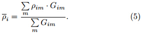
Only AMVs derived for the Northern Hemisphereare compared with the radiosonde wind field becauseof the general lack of radiosonde stations in the SouthernHemisphere. Table 1 presents statistical comparisonsof the AMVs derived from the IR1 and IR3channels before and after height reassignment with radiosondeobservations.
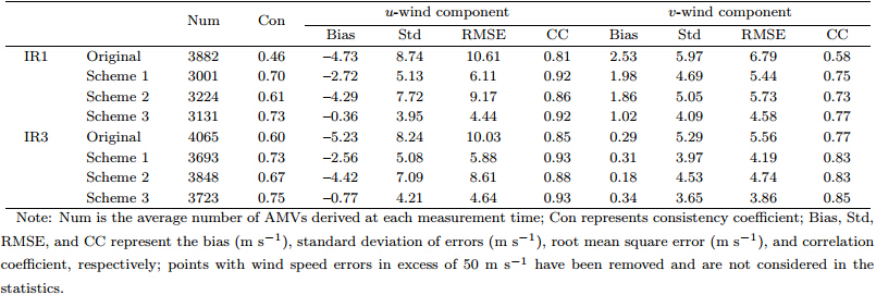 |
The u-wind components of the original IR1 AMVspossess a mean negative bias of –4.73 m s−1, while thev-wind components possess a mean positive bias of2.53 m s−1. The AMVs are improved following heightreassignment by all three schemes. Scheme 3 providesthe largest improvement, Scheme 1 the second largest, and Scheme 2 the smallest. For example, Scheme 3 reducesthe biases in u-wind by 4.37 m s−1, the biases inv-wind by 1.51 m s−1, the st and ard deviation of errorsin u-wind by 4.79 m s−1 and the st and ard deviation oferrors in v-wind by 1.88 m s−1. The correlation coefficientsare improved by 0.11 and 0.19, respectively, theconsistency coefficient by 0.27 and the overall qualityby 58.7%. The number of removed AMVs accounts for19.3% of the total. Some of these AMVs are removedfor reasons other than reassignment, while some AMVremoval can be attributed to the choice of parametersin the schemes. For instance, the horizontal radius ofinfluence R can affect the consistency coefficients betweenAMVs and their surrounding environment; aconsistency coefficient threshold that is set too highcan result in the removal of a large number of AMVsbecause the algorithm fails to find suitable levels towhich to reassign them. An optimized selection ofthese parameters is necessary but highly complicated.
The improvements in IR3 AMVs following reassignmentare similar to those for IR1 AMVs. Scheme 3 reduces the bias in u-winds by 4.46 m s−1. The biasin v-winds is increased; however, the st and ard deviationof errors in v-winds is reduced by 1.64 m s−1, theRMSE is reduced by 1.7 m s−1, and the correlationcoefficient is increased by 0.08. Taken together, theseresults indicate that the quality of the AMV v-winds isalso improved. Scheme 3 improves the consistency coefficientby 0.15 and the overall quality by 25%. Thefraction of removed AMVs is 8.4% of the total, lessthan that for IR1.
The consistency coefficient and RMSE indicatethat the quality of the AMVs derived from IR3 is initiallybetter than the quality of those derived fromIR1. The AMVs derived from the two channels aresimilar in quality after height reassignment, but moreAMVs are removed for IR1 than for IR3.3.2.3 Changes in the vertical distribution of AMVs
Figure 4 shows the quantitative vertical distributionof AMVs(represented as percentages of the total)before and after height reassignment. The quantitativevertical distributions of the original IR1 and IR3AMVs are different, consistent with the different altitudesensitivities of the two channels. IR3 detects particlesmainly between 500 and 150 hPa, with greatestsensitivity at 300 hPa; IR1 is most sensitive to particlesat 200–100- and 600–850-hPa levels. The quantitativevertical distributions of AMVs change considerablyfollowing reassignment regardless of the readjustmentscheme.
 |
| Fig. 4. Quantitative vertical distributions of AMVs before and after height reassignment. Unit: percentage relative tothe total number of AMVs integrated over all heights. |
All three reassignment schemes increase the numberof IR3 AMVs assigned to heights at and below500 hPa, indicating that the originally assigned heightswere biased high. The increase in AMVs at and below500 hPa using Scheme 3 is larger than that usingScheme 1, which in turn is larger than that usingScheme 2. Scheme 3 increases the fraction of AMVsassigned to heights at and below 500 hPa from lessthan 10% of the total to over 30% of the total. Yanget al.(2012)found that the bias and the st and ard deviationof errors for IR3 AMVs both peak at around300 hPa. IR3 AMVs are removed in the greatest numbersfrom this level during height reassignment(in Fig. 4), further justifying the reassignment scheme.
The number of IR1 AMVs at high levels(200–100hPa)is reduced significantly by height reassignment.Approximately 5% of these AMVs are reassigned toheights higher than 100 hPa, but most of them arereassigned to heights within the 500–200 hPa. Thefraction of AMVs assigned to heights near 850 hParemains large and roughly constant after height reassignment.Scheme 3 reassigns the greatest number ofAMVs from the 200–100-hPa layer to middle layers.
Comparison between the IR1 and IR3 AMVsindicates that, although the vertical distribution ofAMVs changes following height reassignment, theheight ranges where IR1 and IR3 feature stronger sensitivityremain the same.
The combined AMVs derived from both channels(red line in Fig. 4)are more evenly distributed inheight following height reassignment. If the above resultsare used to assess the quality of the AMVs followingreassignment by each of the three schemes, thenthe higher the quality of the AMVs, the more evenlythose AMVs are distributed in vertical space. Thevertical distribution of AMVs following height reassignmentis more consistent with the statistical distributionof water vapor.4. AMV height reassignment using NWP wind
The previous section discusses AMV height reassignmentusing the NCEP/FNL analysis wind field asa reference. This wind field is an accurate referencethat enables high-quality reassignment, and it is suitablefor discussing the reassignment schemes and creatingAMV reanalysis data; however, height reassignmentduring operational derivation of AMVs cannotbe accomplished using this wind field. In operationalapplications, the wind field from a numerical modelforecast can be used as a reference. These forecastfields are not so accurate as the analysis fields; thefeasibility of the above methods in the operationalderivation of AMVs must therefore be assessed independently.
The wind field forecast from the T511 Global AviationMid-range Numerical Weather Prediction Systemis used as a reference. This forecast has a horizontalresolution of 1°×1° and a vertical resolution of 17layers. The T511 system produces global mid-rangenumerical weather forecast products with a validityperiod of 10 days and an applicable validity period of6 days at 0000 and 1200 UTC everyday. These midrangeforecasts are of favorable accuracy2 .
The 12-, 24-, 48-, 72-, 96-, and 120-h forecastfields from the T511 system are used to reassign theheights of AMVs at a total of 114 times ranging from0000 UTC 2 September to 1200 UTC 30 September2009. The results presented in Section 3 indicate thatScheme 3 outperforms the other two schemes and thatthe quality of the IR3 AMVs is better than the qualityof the IR1 AMVs; consequently, this section only considersoperational height reassignment of IR3 AMVsusing Scheme 3.
Figure 5 presents a comparison of the IR3 AMVsbefore and after height reassignment with NCEP/FNLwind. Regardless of the length of the forecast used asa reference, the quality of the AMVs following heightreassignment is better than the quality of AMVs beforeheight reassignment. Moreover, shorter forecastperiods provide higher-quality revised AMVs, indicatingthat the quality of the forecast fields deteriorateswith the length of the forecast. Using the 12-h forecastfield improves the consistency coefficient from 0.5–0.6to approximately 0.75. The RMSEs of the u-wind arereduced from over 8 to about 4 m s−1 and the RMSEsof the v-wind are reduced from over 5 to about 3–4m s−1, with the overall quality improved by approximately25%–50%. In addition, the magnitude of thetemporal fluctuations in the AMV errors is reduced and the seasonality in these errors is largely removed.
 |
| Fig. 5. A comparison of AMV wind speeds derived from the water vapor channel before and after forecast windheight reassignment with NCEP/FNL data.(a)Consistency coefficients, (b)RMSEs of zonal winds, and (c)RMSEs ofmeridional winds. |
The improvement in derived AMVs followingheight reassignment with the T511 forecast field asa reference is further verified by comparison with radiosondedata. Figure 6 shows the vertical profiles ofbiases and RMSEs in AMV wind speeds before and after height reassignment.
 |
| Fig. 6. Vertical distributions of statistical errors in wind speed before and after height reassignment for AMVs derivedfrom the water vapor channel.(a)Biases of zonal wind, (b)RMSEs of zonal wind, (c)biases of meridional wind, and (d)RMSEs of meridional wind. Height reassignment is accomplished using either T511 12-h forecast winds or NCEP/FNLreanalysis winds as indicated in the legend; errors are calculated relative to radiosonde observations. |
Using the T511 12-h forecast as a reference forheight reassignment reduces negative biases in theoriginal AMV u-winds in the layers of 500 hPa and above, and reduces positive biases in the original AMVu-winds at 700 hPa. Height reassignment using T51112-h forecast winds slightly underperforms that usingNCEP/FNL winds under Scheme 3, but outperformsthat using NCEP/FNL winds under Scheme 1or Scheme 2. The RMSEs in u-winds throughout the700–250-hPa layer are similar in magnitude to thoseachieved using NCEP/FNL winds under Scheme 3.
Height reassignment using the T511 12-h forecastreduces positive biases in v-winds at 300 hPa and below, but does not substantially reduce biases above 300hPa. The biases at 150 hPa are actually larger followingheight reassignment. Nevertheless, the reductionsin RMSEs indicate that the quality of the v-winds isgreatly improved following height reassignment. Asfor the u-winds, height reassignment using the T51112-h forecast winds slightly underperforms that usingNCEP/FNL winds under Scheme 3, but is superior tothat using NCEP/FNL winds under Scheme 1 orScheme 2.
The effectiveness of AMV height reassignment usingthe T511 forecast field as a reference is furtherquantified by the statistics presented in Table 2. Themean bias in AMV u-winds is reduced by 3.75 m s−1, the st and ard deviation of errors is reduced by 4.04 ms−1, and the RMSE is reduced by 5.42 m s−1 followingheight reassignment, while the correlation coefficient isincreased by 0.1. The mean bias in AMV v-winds isincreased by 0.13 m s−1, but the st and ard deviationof errors and RMSE are reduced by 1.62 and 1.71 ms−1, respectively. The correlation coefficient for AMVv-winds is increased by 0.08, indicating that the qualityof the v-winds is also improved by height reassignment.The consistency coefficient is increased by 0.16 and the overall quality is improved by 26.7%; theseimprovements are similar to those effected by applyingScheme 3 with NCEP/FNL winds as the reference.
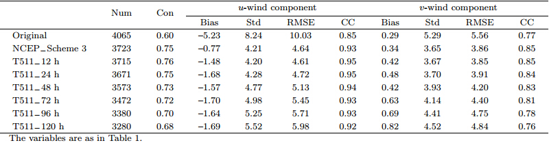 |
The quality of reassigned AMVs decreases slowlybut linearly with the length of the forecast used as thereference wind field. Relative to AMVs revised usingthe 12-h forecast, AMVs revised using the 120-h forecasthave larger biases in both u-wind(by 0.21 m s−1) and v-wind(by 0.4 m s−1), larger st and ard deviationsof errors(by 1.32 and 0.85 m s−1, respectively), and smaller correlation coefficients(by 0.03 and 0.09, respectively).The consistency coefficient also decreasesby 0.08 when the 12-h forecast is replaced by the 120-hforecast. The quality of the AMVs is still improvedrelative to the original AMVs(by 13%). Furthermore, using longer forecast periods results in less highqualityAMVs following height reassignment. An increaseof 24 h in the forecast length results in a reductionof approximately 100 AMVs in the final product.These results indicate that the quality of the forecastfield is reduced as the length of the forecast period isextended. This reduction in the quality of the referencereduces the number of AMVs that can be reassignedto suitable layers.
The above analysis suggests that the accurateNWP wind fields can be used for height reassignmentin the operational derivation of AMVs. The forecastwinds are more helpful and the height reassignmentis more effective when the forecast period is shorter.Forecast fields with longer validity periods still providevaluable information when used for height reassignment, but result in the removal of more high-qualityAMVs.5. Conclusions and discussion
Yang et al.(2012)analyzed the characteristics ofthe distribution of errors in AMVs derived from theFY-2C satellite. They noted that the major source ofthese errors is AMV height assignments that are toohigh, and suggested a proto-type height reassignmentmethod. This paper has explored the rationale and technical details of this height reassignment method.Three schemes for height reassignment using a referencewind field have been designed and presented, along with a method of quality control. The conclusionsare as follows.
(1)The case study using NCEP/FNL reanalysiswind data as a reference shows that some mismatchedor disorderly winds are removed or reassigned to otherlayers. The height reassignment improves the detailedrepresentation of the wind field, and the directions and speeds of AMVs better coincide with radiosonde observationsfollowing height reassignment.
(2)The quality of the derived AMVs is generallyimproved by all of the reassignment algorithms.Scheme 3 boasts the best quality and stability, outperformingScheme 1, which in turn is better than Scheme 2. Height reassignment using Scheme 3 betterrepresents the true state and allows the diagnosis ofbias sources. This height reassignment algorithm willhelp the AMV derivation group to identify sources ofbias and ways to improve the data quality of satellitederivedAMVs.
Statistical analysis of the AMVs revised usingNCEP/FNL data indicates that the negative biasesin u-wind speeds are reduced from [–5, –4] m s−1 to<–1 m s−1. The quality of the AMV v-winds is alsoimproved. The amplitude of temporal error fluctuationsis substantially reduced, and seasonal changesin mean errors are largely removed. The consistencycoefficient between IR1 AMVs and the radiosondewinds increases by 0.27 following height reassignment;the overall quality increases by 58.7%. The consistencycoefficient between IR3 AMVs and radiosondewinds increases by 0.15, with a jump in overall qualityof 25%. These improvements indicate that adjustingAMV heights without changing wind speeds ordirections can effectively improve the precision and stability of the data products.Height reassignment increases the fraction of IR3AMVs assigned to heights at 500 hPa or below, whilesignificantly reduces the fraction of AMVs assignedto heights at 300 hPa or above. A large number ofIR1 AMVs are reassigned from the upper troposphere(200–100 hPa)to the middle troposphere(500–200hPa). The number of AMVs assigned to lower layersdoes not change dramatically. These results areconsistent with the underst and ing that the heightsassigned to AMVs are generally too high.
(3)Experimental operational height reassignmentusing T511 12-h forecast as the reference wind fieldreduces negative biases in IR3 u-winds at 500 hPa and above and positive biases in v-winds at 300 hPa and below. The consistency coefficient between the AMVs and the radiosonde wind field increases by 0.16. Thequality of the AMVs is improved by 26.7%, comparableto the improvement in quality effected by usingNCEP/FNL winds under Scheme 3 and better thanthe improvements effected by using NCEP/FNL windsunder Scheme 1 or Scheme 2.
As the length of the NWP forecast used as thereference increases, the improvement in AMV qualityprovided by height reassignment decreases slowly and linearly. The quality of the revised AMVs is still improvedby 13% when the 120-h forecast is used, but alarger number of valid AMVs is removed.
The error in height assignment is not the onlyerror that affects the accuracy of satellite-derivedAMVs. It is of great importance to better determineboth the direction and speed of horizontal windvectors(Velden and Bedka, 2008; von Bremen et al., 2008). Furthermore, the schemes presented here aresuitable for wind fields that vary relatively smoothlywithin a given horizontal range. For wind fields withsharp gradients, such as at the edge of a jet, the consistencycoefficient is unable to provide a quantitativemeasure of consistency with the ambient wind field.This difficulty could affect the effectiveness of heightreassignment using this type of algorithm. A numberof other outst and ing challenges, such as optimizationof the scheme parameters, also deserve in-depth study.
Acknowledgments. The authors wish to thankDr. Jing Li and Dr. Zhao Suxuan for helpful discussions.
| [1] | Borde, R., and R. Oyama, 2008: A direct link between feature tracking and height assignment of operational atmospheric motion vectors. The 9th International Winds Workshop, Annapolis, Maryland, USA, 1–8. |
| [2] | Chen Hua, Xu Jianmin, Zhang Qisong, et al., 1999: The quality controlling of cloud winds using height updating. Scientia Meteor. Sinica, 19(1), 20–25. (in Chinese) |
| [3] | Diner, J. D., P. G. Asner, R. Davies, et al., 1999: New directions in earth observing: Scientific applications of multi-angle remote sensing. Bull. Amer. Meteor. Soc., 80, 2209–2228. |
| [4] | Hasler, A. F., 1981: Stereographic observations from geosynchronous satellites: An important new tool for the atmospheric sciences. Bull. Amer. Meteor. Soc., 62, 194–212. |
| [5] | Li Yanbing, Huang Sixun, and Zhai Jingqiu, 2009: A review of satellite wind retrieval technologies. Scientia Meteor. Sinica, 29(2), 277–284. |
| [6] | Menzel, W. P., W. L. Smith, and T. R. Stewart, 1983: Improved cloud motion wind vector and altitude assignment using VAS. J. Climate Appl. Meteor., 22, 377–384. |
| [7] | Nieman, S., J. Schmetz, and P. Menzel, 1993: A comparison of several techniques to assign heights to cloud tracers. J. Appl. Meteor., 32, 1559–1568. |
| [8] | Rohn, M., G. Kelly, and R. W. Saunders, 2001: Impact of a new cloud motion wind product from METEOSAT on NWP analyses and forecasts. Mon. Wea. Rev., 129, 2392–2403. |
| [9] | Schmetz, J., and K. Holmlund, 1992: Operational cloud motion winds from METEOSAT and the use of cirrus clouds as tracers. Adv. Space Res., 12(7), 95–104. |
| [10] | Steinhoff, D. F., 2009: A contemporary review of the production and utility of atmospheric motion vectors, Geography 820 Term Paper, 1–38. |
| [11] | Szejwach, G., 1982: Determination of cirrus cloud temperature from infrared radiances: Application to METEOSAT. J. Appl. Meteor., 21, 284–293. |
| [12] | Velden, C. S., and K. Bedka, 2008: Identifying the uncertainty in determining satellite-derived atmospheric motion vector height attribution. The 9th International Winds Workshop, Annapolis, Maryland, USA, 63–74. |
| [13] | von Bremen, L., N. Bormann, S. Wanzong, et al., 2008: Evaluation of AMVs derived from ECMWF model simulations. The 9th International Winds Workshop, Annapolis, Maryland, USA, 9–18. |
| [14] | Wu, Q. X., 1993: Computing velocity field from sequential satellite images. Satellite Remote Sensing of the Oceanic Environment. Jones, Sugimori, and Stewart, Eds., Seibutsu Kenkvusha Co. Ltd., 38–47. |
| [15] | Xu Jianmin, Zhang Qisong, and Fang Xiang, 1997: Height assignment of cloud motion winds with infrared and water vapour channels. Acta Meteor. Sinica, 55(4), 408–417. (in Chinese) |
| [16] | —–, —–, —–, et al., 1998: Cloud motion winds from FY-2 and GMS-5 meteorological satellites. The 4th International Winds Workshop, Saanenmoser, Switzerland, EUMETSAT Publication, EUM P24, 41–48. |
| [17] | Xue Jishan, 2009: Scientific issues and perspective of assimilation of meteorological satellite data. Acta Meteor. Sinica, 67(6), 903–911. (in Chinese) |
| [18] | Yang Chengyin, Lu Qifeng, Wu Xuebao, et al., 2012: Error analysis for atmospheric motion vectors of FY-2C. J. Infrared Millim. Waves, 31(1), 73–79. (in Chinese) |
| [19] | Zapotocny, T. H., J. A. Jung, J. F. Le Marshall, et al., 2008: A two-season impact study of four satellite data types and rawinsonde data in the NCEP Global Data Assimilation System. Wea. Forecasting, 23, 80–100. |