 2012, Vol. 26
The Chinese Meteorological Society
Article Information
- LIU Hailong, LIN Pengfei, YU Yongqiang and ZHANG Xuehong. 2012.
- The Baseline Evaluation of LASG/IAP Climate System Ocean Model (LICOM) Version 2
- J. Meteor. Res., 26(3): 318–329
- http://dx.doi.org/10.1007/s13351-012-0305-y
-
Article History
- Received April 30, 2011
- in final form Feburary 9, 2012


The first effort to develop a global ocean generalcirculation model(OGCM)in the State Key Laboratoryof Numerical Modeling for Atmospheric Sciences and Geophysical Fluid Dynamics/Institute of AtmosphericPhysics(LASG/IAP)can be traced back to the1980s. The primary motivation for developing such anOGCM is to build a coupled atmosphere-ocean model,as well as to study the ocean circulation. Since the first4-layer,baroclinic OGCM has been established in thelater 1980s(Zhang and Liang, 1989),the family ofLASG/IAP ocean models has been exp and ed in successionduring the past 20 years. The LASG/IAP Climatesystem Ocean Model(LICOM; Liu et al., 2004a,b)was developed based on the third version of theLASG/IAP OGCM(Jin et al., 1999). As its previousversions,the intermediate resolution(1 degree)LICOM version 1(LICOM1)was also the oceanic componentof the LASG/IAP climate system model namedFlexible Global Ocean-Atmosphere-L and System version1(FGOALS1)(Yu et al., 2011). FGOALS1 hasparticipated in the Coupled Model IntercomparisonProject phase 4(CMIP4) and has been cited by theFourth Assessment Report(AR4)of the IntergovernmentalPanel on Climate Change(IPCC)(Solomon et al., 2007).
In the past several years,we aimed at reducingthe uncertainties of the upper layer temperature inLICOM1,because it is crucial not only for the surfaceheat fluxes determining the long-term behavior of thewhole climate model,but also for simulating air-seainteraction associated with climate variability on seasonalto interannual timescales. Various key physicalprocesses in LICOM1 have been improved,includingthe vertical turbulent mixing scheme,the solar radiationpenetration scheme(Lin et al., 2007),the advectionscheme(Xiao and Yu, 2006), and the upperlayer taping scheme in the mesoscale eddy parameterization.Besides,the meridional resolution between10°S and 10°N(Liu et al., 2004a) and the vertical resolutionin the upper 150 m(Wu et al., 2005)are alsoincreased to better resolve the equatorial wave-guide and the tropical thermocline,respectively. The detailof those improvements is shown in Appendix A.
Recently,all these improvements are put into version2 of LICOM(LICOM2) and the latest version(version 2)of FGOALS(FGOALS2). The latter is takingpart in the core experiments of CMIP phase 5 forthe Fifth Assessment Report(AR5)of IPCC. The purposeof the present study is to document the baselineperformance of the intermediate resolution(approximate1 degree),st and -alone LICOM2 in simulating thewater properties and the large-scale circulation by usingmetrics from Griffies et al.(2009). The evaluationaims to quantify the uncertainties of LICOM2 againstthe observation and to help us further underst and theperformance of the coupled model in the historical and projection experiments. Attempts were also made toattribute the causes of the biases in LICOM2.
The rest of the paper is organized as follows. Section2 describes the control experiment and the observationaldata. Comparisons of essential metrics betweenLICOM2 and observation are provided in Section3. Section 4 presents concluding remarks.2. Control experiment and observational data2.1 Control experiment
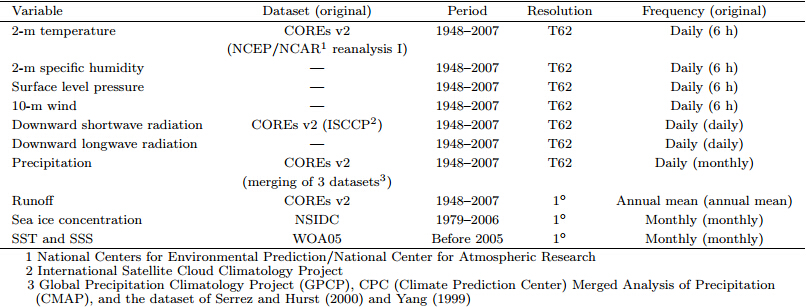
The Community Climate System Model(CCSM)formula and the dataset prepared by Large and Yeager(2004),which are suggested as the only forcing method and forcing dataset for the Coordinated Ocean-ice ReferenceExperiments(COREs; Griffies et al., 2009),areadopted in the present study. Therefore,the resultsfrom LICOM2 can be compared with the results fromCORE models. In Large and Yeager formula(Large and Yeager, 2004),the surface turbulent fluxes arecomputed by the atmospheric state variables,includingthe 10-m air temperature,10-m specific humidity,sea level pressure,10-m wind speed, and vectors of 10-m wind. The downward solar radiation and the downwardlongwave radiation fluxes are both obtained fromthe observation. Albedo of 5.5% is used to computethe net surface shortwave radiation. The net longwaveradiation is computed by the observed downward longwaveradiation minus the blackbody radiation of thesimulated sea surface temperature(SST). All these observationaldata are from the corrected Normal YearForcing(NYF)data of COREs version 2(Large and Yeager, 2004).
Virtual salinity flux is employed as the boundarycondition for the salinity. The reference salinityis taken as 35 psu. Precipitation,evaporation, and river runoff are also from the observational dataset of Large and Yeager(2004). Besides,an extremely weakrestoring term with the piston velocity of 12.5 m yr−1is applied in this experiment to restore the sea surfacesalinity(SSS)to the observation.
Because the ocean–only model is used in thepresent study,observed sea ice concentration from theNational Snow and Ice Data Center(NSIDC)of USover 1979–2006 is used in LICOM2. The temperature and salinity under the sea ice layer are restored to theobservation from World Ocean Atlas 2005(WOA05;Locarnini et al., 2006; Antonov et al., 2006)with atimescale of 30 days. Temperatures lower than the icepoint(–1.8℃)are simply set to the ice point. To testthe model sensitivity to the sea ice concentration data,an experiment using the data from the Hadley Centreof Met Office over 1948–2007 is also conducted.
The present study aims to investigate the climatologicalmean state of ocean in LICOM2. Therefore,following COREs phase 1,we conducted the experimentfrom the initial condition with WOA05 temperature and salinity and no current,forced by repeatingthe daily corrected NYF of Large and Yeager(2004).More details about the forcing data can be found inTable 1. LICOM2 has been integrated for 500 yr toallow the deep circulation to reach a quasi-equilibriumstate. The climatology for analysis is computed overthe last 10 years(491–500)of integration.
Three datasets are used here. First,potentialtemperature and salinity from WOA05(Locarnini et al., 2006; Antonov et al., 2006)are employed to evaluatethe simulated surface and sub-surface temperature and salinity. Second,meridional heat transport from Ganachaud and Wunsch(2003)is used for comparisonwith the simulation. Third,potential temperature and zonal current in the equatorial Pacific from Johnson etal.(2002)are used to evaluate the results of LICOM2.3. Results
In addition to the forcing formulation and dataset,Griffies et al.(2009)proposed a set of metricsto evaluate ocean models. Here,we pick sevenprimary metrics to evaluate LICOM: the horizontalaveraged potential temperature and salinity,SST and SSS,the maximum mixed layer depth(MLD),the zonal averaged potential temperature and salinity,the meridional overturning stream-function,polewardheat transport(PHT), and the currents and thermoclinein the tropical Pacific. Since there is no sea icemodel,the sea ice variables are not included in thepresent study.3.1 Horizontal averaged potential temperature and salinity
Figure 1 shows the anomalous annual mean temperature and salinity of LICOM2 as a function ofdepth and time against observations from WOA05.A detailed vertical structure and the evolution of themodel drift are revealed. It is seen that a rapid adjustmentoccurs in the first 50 years. After that time,thetemperature and salinity above 500 m reach a quasiequilibriumstate with cold and fresh water in the uppermixed layer and warm and fresh water in the tropicalthermocline. Below 500 m,the temperature and salinity drift gradually after the first 50-yr integration, and the salinity has a slight trend even in the last 50-yr integration. This suggests that longer integrationis needed to reach an equilibrium state in the deeperocean.
 |
| Fig. 1. Horizontal averaged drift of the annual mean(a)potential temperature(℃) and (b)salinity(psu)as a functionof depth and time for LICOM2. The observation is from Locarnini et al.(2006)for(a) and Antonov et al.(2006)for(b). |
The magnitudes of the model biases are about0.6℃ and 0.2 psu for temperature and salinity,respectively.The biases are comparable with the zcoordinatemodel presented in Griffies et al.(2009),such as the Parallel Ocean Program(POP; about 1.5℃ and 0.2 psu) and the Modular Ocean Model(MOM;about 1℃ and 0.1 psu).
The patterns of errors in temperature and salinityfrom LICOM2 are different from those from the COREmodels. Because the forcing formulation and datasetare similar,the errors may be caused by the differenceof the model physical processes,such as the parameterizationof diapycnal mixing and isopycnal mixingdue to mesoscale eddy. These were also suggested by Griffies et al.(2009). The absence of the sea ice modelis also a possible reason for different patterns of modeldrift.3.2 SST and SSS
Figure 2a shows the SST differences between LICOM2 and WOA05. In general,LICOM2 presentslarge warm biases with the area average of 0.32℃ inthe tropics(20°S–20°N) and 0.64℃ in the latitudessouth of 60°S. In the subtropics(20°–60°),there areslight cold biases due to the large cold and warm biasesalong the major fronts,such as the regions aroundthe Kuroshio,the Gulf Stream, and the Antarctic CircumpolarCirculation(ACC),which are cancelled outwith each other. The Arctic region also shows a slightwarm bias.
 |
| Fig. 2.(a)Sea surface temperature(℃; contour) and the difference between LICOM2 and observation from Locarniniet al.(2006)(℃; shaded), and (b)as in(a),but for sea surface salinity(psu). The observation is from Antonov et al.(2006). |
In the tropics,there appears a large warm bias of1℃ along the east coast of Pacific and Atlantic Ocean and a relatively small warm bias of 0.5℃ in the wholewestern Pacific and eastern Indian warm pool region.The former is a common problem for the st and -aloneOGCM, and it is amplified in the coupled model,themechanism of which has been systematically investigatedin some recent studies(e.g.,De Szoeke and Xie, 2008; Zheng et al., 2011). Besides the large solar radiationdue to the lack of low stratocumulus clouds,theweak coastal upwelling is the direct cause of the warmbiases. For the OGCM,both the errors in the surfacewind data and the coarse resolution may lead to theweak upwelling in this region.
Another common bias in the tropics is the exaggeratedequatorial Pacific cold tongue. This is firstpointed out by Stokdale et al.(1993) and is a longlastingproblem. Because the mixed layer heat budgetof the cold tongue is dominated by the ocean dynamics,the errors in the vertical heat transport may bethe primary cause of the cold bias. Recent studies alsoindicate that the lack of eddy heat transport by thetropical instability wave(TIW)can partly contributeto the spurious strong cold tongue(e.g.,Jochum and Murtugudde, 2006).
In the region south of 60°S,LICOM2 exhibits alarge warm bias. This is not common for the COREmodels. As shown in the following subsections,thewarm anomaly can be found below the surface. Therefore,the meridional density gradient,which drivesACC,is largely reduced. In the early experiments ofLICOM2,the volume transport across the Drake Passageis only 81 Sv(Sv = 106 m3 s−1),about half ofthe observation of about 130 Sv(e.g.,Cunningham et al., 2003). Because the surface forcing in LICOM2 isthe same as the CORE models,the warm bias shouldbe due to the internal physical processes in LICOM2.
According to previous studies(e.g.,Gent et al., 2001),two sets of sensitive experiments are conductedto underst and the causes of the warm bias. First,wetest the sensitivity of the sea ice concentration on thewarm bias. Two climatology datasets are chosen: oneis from NSIDC over 1979–2006 and the other from theHadley Centre of Met Office over 1948–2007. Figure 3shows the annual mean difference of sea ice concentration and SST between the two experiments. Aroundthe Antarctic,the value of Hadley Centre data is largerthan that of NSIDC. This results in less surface fluxreleased and higher warm bias in the experiment usingthe Hadley Centre data. Second,the sensitivityof mesoscale eddy parameterization of Gent and McWilliams(1990)on the warm bias and the magnitudeof ACC has been investigated by two experimentsusing different isopycnal( and thickness)mixingcoefficients of 500 and 1000 m−2 s−1,respectively.Same as in Danabasoglu and McWilliams(1995),thesmaller mixing coefficient is associated with strongerACC and a smaller warm bias(figure omitted). Thisindicates that the improper mixing coefficient of themesoscale eddy parameterization may also contributeto the warm bias in the Southern Ocean.
 |
| Fig. 3. The differences of(a)sea ice concentration(%) and (b)SST(℃)for two sensitive experiments using prescribedsea ice data from the Hadley Centre of Met Office and NSIDC. |
Except for the above two factors,the missingbrine rejection process is also considered as an additionalfactor that causes the warm bias. This processmay greatly reduce the vertical mixing and deep convection, and then weaken the overturning circulation.These are all conducive to a warm SST bias in theSouthern Ocean. But further sensitive experimentsare needed to investigate this process.
Figure 2b shows the SSS differences between LICOM2 and WOA05. In the present experiment,althoughonly a weak restoring term is included in theboundary condition of salinity in the open ocean,LICOM2simulates SSS reasonably. Except for the region related to the western boundary currents and nearthe mouth of rivers,the biases in most regions arebelow 0.5 psu(Fig. 2b). This magnitude is comparablewith that in CORE models(Griffies et al., 2009).This indicates large uncertainties in the runoff data ofCORE dataset and should be improved further.3.3 Maximum MLD
Figure 4 shows the maximum MLD for the climatologyof WOA05 and LICOM2. Following De BoyerMontégut et al.(2004),MLD here is defined as thedepth of the isothermal 0.2℃ lower than the temperatureat 10 m. MLD is primarily determined bythe wind stirring and the static instability associatedwith surface buoyancy fluxes. The maximum MLD occursduring wintertime,when the surface water is coldby heat loss due to the turbulent fluxes and strongwind stirring. These processes are crucial for the watermass formation and the thermohaline circulation.Therefore,the maximum MLD is an important metricsto evaluate the ability of an ocean model to simulatethese processes.
 |
| Fig. 4. The maximum mixed layer depth for the climatology of(a)WOA05 observation(Locarnini et al., 2006) and (b)LICOM2 simulation. |
The sophisticated vertical mixing scheme and therelatively fine vertical resolution lead to a good simulationof MLD in LICOM2 in the tropics,especiallyin the shallow MLD region,including eastern equatorialPacific off the western coast of Costa Rica and thesouthwestern equatorial India. In the region betweenthe subtropics and subpolar gyre,MLD is much overestimatedagainst WOA05. More heat would subductinto the tropical thermocline around 200 m. As shownin Fig. 1a,warm temperature anomaly can be foundaround this depth.
The discrepancies between LICOM2 and the observationcan also be found in Antarctic. In LICOM2,the deep mixed layer is separated in smallpatches,while in observation,the distribution of thedeep mixed layer is an integrated belt. As mentionedin the previous subsection,the mixing under the seaice is supposed to be much underestimated in LICOM2in Antarctic mainly due to the missing of the brinerejection or the largely overestimated sea ice concentration.3.4 Zonal averaged potential temperature and salinity
Figure 5 shows the zonal averaged temperature and salinity from LICOM2(contour) and the differencebetween LICOM2 and WOA05(shaded). Becausethe related distribution is directly set by theglobal thermohaline and wind-driven circulation and is simple to obtain,this is a popular method to evaluateOGCM. Like the CORE models,the biases ofLICOM2 in temperature and salinity are less than 1℃ and 0.2 psu over the most latitude-depth planes.
 |
| Fig. 5.(a)Zonal averaged potential temperature(℃; contour) and the difference(℃; shaded)between LIOM2 and WOA05(Locarnini et al., 2006).(b)As in(a),but for sea surface salinity(psu). The observation is from Antonov et al.(2006). |
Comparison between Figs. 1a and 5a shows fivedifferent layers with warm biases in the tropical thermocline and around 2500 m, and cold biases at the surface,in the permanent thermocline, and at the oceanbottom. Figure 5a clearly shows the connection betweenthe sub-surface biases and the processes at thesurface: the warm anomalies in the tropical thermoclinearound 10° and 30°N are associated with theoverestimated MLD in the North Pacific and AtlanticOcean,the cold biases in the permanent thermoclineare connected with the cold SST biases in the subtropics, and the warm deep water around 2500 m is relatedto the warm biases in the polar regions. Theseresults suggest that the surface forcing and the mixedlayer processes are important for simulation of the subsurfacewater temperatures.
We can also find the similar relationship,but withfewer layers in the salinity field(Fig. 5b): the freshupper layer(above 700 m),the salty main thermocline, and the fresh bottom layer. The extremely fresh biasin the upper layer can be found in the Arctic. Thisis associated with both runoff and sea ice processes,which have large uncertainties in the experiment. Thesalty bias in the thermocline also primarily occurs inthe Arctic. The other two large warm biases appeararound 40°S and 40°N. The former is associated withthe salty water in the Southern Ocean; the latter isrelated to the salty water overflow from the Mediterranean(figure omitted).
We notice that the large biases in Fig. 5 mainlyappear in the polar regions. Therefore,we suspectthat these biases may be related to the prescribed seaice concentration. Further experiments with LICOM2coupled to a sea ice model forced by CORE data areundergoing to underst and the mechanism of the biases.Compared with the CORE models,the warm and salty biases around the Antarctic continent are relativelylarge in LICOM2,especially the warm biases.These biases reduce the meridional density gradient and weaken the transport of ACC. The volume transportthrough the Drake Passage is about 81 Sv in thelast 10 years,which is still about 40% smaller than theobservation. Besides the sea ice or mixing processes,this bias is possibly related to the entire thermohalinecirculation simulation deficiency as suggested by Russell et al.(2006).3.5 Meridional overturning stream-function
The meridional overturning stream-function iscommonly used to present the features of meridionaloverturning circulation(MOC). Figure 6 shows themeridional overturning stream-function over the globe and in Atlantic simulated by LICOM2. LICOM2 capturesthe primary cells very well: the two vigorouswind-driven cells in the tropics,the Deacon Cell between40° and 60°S,the North Atlantic Deep Water(NADW)above 3000 m north of 40°S,the bottomcell between 20° and 40°S, and the Antarctic BottomWater(AABW)adjacent to Antarctic are all clearlyshown in Fig. 6.
 |
| Fig. 6.(a)Global and (b)Atlantic meridional overturning stream-function(Sv = 106 m3 s−1)for LICOM2. |
The volume transport of the Deacon Cell in LICOM2is about 25 Sv,comparable with the otherz-coordinate model results shown in Griffies et al.(2009). But it penetrates much deeper than that inthe CORE models, and cuts off the connection betweenAABW and the bottom cell. This reduces themagnitude of both AABW and the bottom cell. Asshown in previous subsection,the deep Deacon Cell and the weak AABW may be related to the warm and salty biases around the Antarctic.
Unlike temperature and salinity,there is no directlyobservation of the MOC. Recently,an observingsystem for the MOC at 26.5°N in the Atlantic is developedunder the Rapid Climate Change(RAPID)Programmeof the Natural Envioronment Research Council,UK. The observed transport is 18.5 Sv averagedover 2004–2009,4–5 Sv larger than the simulation ofLICOM2 at the same latitude.3.6 PHT
The PHT by the ocean,which is a part of thetotal heat transport,is primary driven by the differenceof the solar heating between the tropics and thepolar region. It is critical for the equilibrium of theclimate system. Figure 7 shows the simulated PHTfor globe and Atlantic. The dots are estimations(regardedas observations)from Ganachaud and Wunsch(2003). The total heat transport is a composite ofthree terms: the PHT due to the mean circulation,the PHT due to the mesoscale eddy, and the PHTdue to diffusivity. The global PHT is about 1.5 PWin the Northern Hemisphere and about 1 PW in theSouthern Hemisphere. These values are close to theobservation. The simulation is much smaller than theobservation in the Atlantic,especially between 20°S and 20°N. The weak heat transport is also the commonproblem for intermediate resolution OGCMs.
 |
| Fig. 7.(a)Global and (b)Atlantic polarward heat transport(PHT; PW = 1015 W)for LICOM2(solid). The dots areestimations from Ganachaud and Wunsch(2003). |
The performance of the ocean model in tropicalPacific is essential for the coupled model to simulatethe interannual variability. Therefore,the thermocline and the circulation in the equatorial Pacific are alsothe common variables to evaluate an OGCM. Figure 8 shows the temperature along equatorial Pacific forthe observation from Johnson et al.(2002) and forLICOM2. The warm bias in the warm pool and coldbias in the cold tongue,which are mentioned in subsection3.2,are also clearly seen in Fig. 8. The rise of thetropical thermocline in the eastern Pacific indicatesthat the strong equatorial upwelling causes the coldbias. The tropical thermocline in LICOM2 is morecompact than in the previous version(figure omitted).
 |
| Fig. 8. The potential temperature(℃)along the equatorial Pacific for(a)Johnson et al.(2002) and (b)LICOM2. |
Figure 9 shows the zonal current along the equatorialPacific for the observation from Johnson et al.(2002) and for LICOM2. Through reducing horizontalviscosity from 2×10⁴ to 3×10³ m−2 s−1,the simulatedpattern of zonal current along the equator issignificantly improved. Therefore,the Equatorial UnderCurrent(EUC)in the thermocline is increased to0.7 m s−1. Although the EUC is about 30% less thanthat of observation,this is still a reasonable value foran intermediate resolution OGCM.
 |
| Fig. 9. The zonal current(m s−1)along the equatorial Pacific for(a)Johnson et al.(2002) and (b)LICOM2. |
In the present study,the baseline performance ofthe intermediate resolution,st and -alone OGCM,LICOM2,has been evaluated against the observation byusing main metrics from Griffies et al.(2009). In general,the errors in the water properties and in the circulationare comparable with the CORE models. Somecommon problems of OGCM also appear in LICOM2,such as the cold bias in the eastern Pacific cold tongue,the warm biases off the eastern coast of the basins,theweak poleward heat transport in the Atlantic, and therelatively large biases in the Arctic Ocean. A uniquesystematic bias occurs in LICOM2 over the SouthernOcean compared with CORE models. The biases canbe found in both the stratification and the circulation,such as the warm and salty biases around 2500 m,theweak transport of ACC and the deep penetration ofDeacon Cell. It seems that this bias may be related tothe sea ice process around the Antarctic.
A systematic comparison between LICOM1 and LICOM2 is undergoing. Preliminary results indicatethat the performance of LICOM2 has been substantiallyimproved in many aspects,mainly including theshallow MLD in the eastern Pacific and western India,the small temperature and salinity biases in thedepth-latitude plane,the increasing MOC in the Atlantic,the increasing EUC,etc. The updated verticalmixing scheme,the increase of vertical resolution, and the reduction of the viscosity are all considered to havecontributed to these improvements. But more sensitive experiments are needed to further identify the effectof each process.
In this study,the performance of LICOM2 hasbeen investigated by using an equilibrium simulation.To underst and the model behavior,the abilityof the model in simulating the climatic variabilityon intraseasonal to intradecadal timescales alsoneeds to be further evaluated. This work is alsoundergoing.
The model used in the current study is an oceanonlymodel,rather than an ocean-ice coupled model asthat of the CORE models. The results of this work aretherefore not good for comparison with the results ofCORE models,especially in the high latitudes and fordeep circulations. Because the process related to thesea ice can affect not only the local temperature and salinity,but also the remote region through modifyingthe thermohaline circulation. Thus,the ocean-sea icecoupled experiment is also needed.
Acknowledgments. We thank the two anonymousreviewers for their helpful comments and suggestionsthat have improved the manuscript.Appendix A. Brief description of improvements of LICOM2 from LICOM1
The fundamental framework of LICOM2 is inheritedfrom LICOM1. The primary features includethe η-coordinate,free surface,primitive equation, and mesoscale eddy parameterization from Gent and McWilliams(1990),etc. The main improvementsof LICOM2 are listed in Table A1.
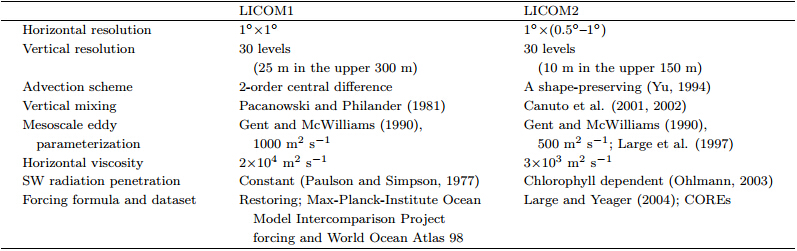
Because of the smaller length scale,which is alwaysmeasured by the first baroclinic Rossby radiusof deformation,in the ocean than that in the atmosphere,the horizontal resolution is crucial for oceancirculation simulation. To better resolve the equatorialwave-guide with an acceptable computational cost,the meridional resolution between 10°S and 10°N hasbeen increased from 1° to 0.5°. The grid distance between10° and 20° gradually varies from 0.5° to 1°.
To improve the simulation of the upper ocean,thevertical level of LICOM has been rearranged following Wu et al.(2005). The number of levels in the upper150 m has been more than doubled,increasing from 6to 15 levels.A.2 Physical processes
Besides the resolution,the physical parameterizationschemes have also been improved in LICOM2.First,the scheme dependent on Richardson number(Pacanowski and Philander, 1981; called PP schemehereafter)for vertical turbulence mixing was replacedby a second-order turbulence closure model of Canutoet al.(2001,2002; called Canuto scheme hereafter).The PP scheme intends to describe the mixing in thetropical thermocline where the mixing is mainly dueto large velocity shear close to EUC. Therefore,thePP scheme is only valid in the tropics,usually from30°S to 30°N. The Canuto scheme is valid globally; itincludes not only the mixing due to the velocity shearbut also the mixing due to the internal-wave break and double diffusion. After using the Canuto scheme,thediscontinuity of water properties between the tropics and extra-tropics has been eliminated since the samevertical mixing scheme is applied over the entire modeldomain. Thus,the horizontal viscosity can be reducedfrom 2×10⁴ to 3×10³ m−2 s−1.
Second,we have modified the mesoscale eddy parameterizationof Gent and McWilliams(1990; calledGM90 hereafter),which is usually used to replace thehorizontal mixing and to correct the spurious diapycnalmixing in the z-coordinate ocean model. Thescheme in LICOM1 is adopted from MOM version 2(Jin et al., 1999)with the isopycnal mixing and thicknessmixing coefficients both assigned to 1000 m−2 s−1, and the maximum slope of isophycnals set to 0.01. Toreduce the mesoscale mixing in the upper layer,theisopycnal and thickness diffusivities have been taperedby the method of Large et al.(1997). Additionally,in order to simulate a stronger Antarctic CircumpolarCirculation(ACC),the isopycnal and thickness mixingcoefficients are reduced from 1000 to 500 m−2 s−1following Danabasoglu and McWilliams(1995).
Third,the two-exponent scheme with constantcoefficients of Paulson and Simpson(1977; calledPS77 hereafter),has been substituted by a scheme of Ohlmann(2003),in which all the parameters are functionsof chlorophyll concentration. Lin et al.(2007)compared the differences of SST between the twoschemes in the eastern equatorial Pacific.
In addition,a shape-preserving advection schemeof Yu(1994)was incorporated into LICOM2 by Xiao and Yu(2006). The excessive equatorial cold tonguehas been significantly reduced due to the improvementof the advection scheme. Therefore,in the presentstudy,we still use the Yu(1994)scheme in the experiment.A.3 Other improvements
There are also improvements in computing techniques and fixing of bugs in LICOM2. These improvementsor corrections are vital for the accuracy and efficiency of the model. The improvements primarilyinclude the following: changing the computationof arrays and variables from single precision to doubleprecision; optimizing the parallel performance;correcting bugs in the restart process,etc. A twodimensionalpartition version of LICOM has also beendeveloped,but only for the eddy-resolving version ofLICOM2 by far.
| [1] | Antonov, J. I., R. A. Locarnini, T. P. Boyer, et al., 2006: World Ocean Atlas 2005, Volume 2: Salinity. NOAA Atlas NESDIS 62, US, Washington D. C., 1–182. |
| [2] | Canuto, V. M., A. Howard, Y. Cheng, et al., 2001: Ocean turbulence. Part I: One-point closure modelmomentum and heat vertical diffusivities. J. Phys. Oceanogr., 31, 1413–1426. |
| [3] | —–, —–, —–, et al., 2002: Ocean turbulence. Part II: Vertical diffusivities of momentum, heat, salt, mass, and passive scalars. J. Phys. Oceanogr., 32, 240–264. |
| [4] | Cunningham, S., S. Alderson, B. King, et al., 2003: Transport and variability of the Antarctic Circumpolar Current in Drake Passage. J. Geophys. Res., 108, 8084–8100. |
| [5] | Danabasoglu, G., and J. McWilliams, 1995: Sensitivity of the global ocean circulation to parameterizations of mesoscale tracer transports. J. Climate, 8, 2967–2987. |
| [6] | De Boyer Mont′egut, C., G. Madec, A. S. Fischer, et al., 2004: Mixed layer depth over the global ocean: an examination of profile data and a profile-based climatology. J. Geophys. Res., 109, C12003, doi: 10.1029/2004JC002378. |
| [7] | De Szoeke, S. P., and Shangping Xie, 2008: The tropical eastern Pacific seasonal cycle: Assessment of errors and mechanisms in IPCC AR4 coupled oceanatmosphere general circulation models. J. Climate, 21, 2573–2598. |
| [8] | Ganachaud, A., and C. Wunsch, 2003: Large-scale ocean heat and freshwater transports during the world ocean circulation experiment. J. Climate, 16, 696–705. |
| [9] | Gent, P., and J. C. Mcwilliams, 1990: Isopycnal mixing in ocean circulation models. J. Phys. Oceanogr., 20, 150–155. |
| [10] | Gent, P. R., W. G. Large, and F. O. Bryan, 2001: What sets the mean transport through Drake Passage? J. Geophys. Res., 106, 2693–2712. |
| [11] | Griffies, S., and Coauthors, 2009: Coordinated ocean-ice reference experiments (COREs). Ocean Modelling, 26, 1–46. |
| [12] | Jin Xiangzhe, Zhang Xuehong, and Zhou Tianjun, 1999: Fundamental framework and experiments of the third generation of IAP/LASG world ocean general circulation model. Adv. Atmos. Sci., 16, 197–215. |
| [13] | Jochum, M., and R. Murtugudde, 2006: Temperature advection by tropical instability waves. J. Phys. Oceanogr., 36, 592–605. |
| [14] | Johnson, G. C., B. M. Sloyan, W. S. Kessler, et al., 2002: Direct measurements of upper ocean currents and water properties across the tropical Pacific Ocean during the 1990s. Prog. Oceanogr., 52, 31–61. |
| [15] | Large, W., G. Danabasoglu, S. Doney, et al., 1997: Sensitivity to surface forcing and boundary layer mixing in a global ocean model: Annual-mean climatology. J. Phys. Oceanogr., 27, 2418–2447. |
| [16] | —–, and S. Yeager, 2004: Diurnal to Decadal Global Forcing for Ocean and Sea-Ice Models: The Data Sets and Flux Climatologies. NCAR/TN-460+STR, 1–105. |
| [17] | Lin Pengfei, Liu Hailong, and Zhang Xuehong, 2007: Sensitivity of the upper ocean temperature and circulation in the equatorial Pacific to solar radiation penetration due to phytoplankton. Adv. Atmos. Sci., 24, 765–780. |
| [18] | Liu Hailong, Zhang Xuehong, Li Wei, et al., 2004a: A eddy-permitting oceanic general circulation model and its preliminary evaluations. Adv. Atmos. Sci., 21, 675–690. |
| [19] | —–, Yu Yongqiang, Li Wei, et al., 2004b: Manual for LASG/IAP Climate System Ocean Model (LICOM1. 0). Science Press, Beijing, 128 pp. (in Chinese) |
| [20] | Locarnini, R. A., A. V. Mishonov, J. I. Antonov, et al., 2006: World Ocean Atlas 2005, Volume 1: Temperature. NOAA Atlas NESDIS 61, US, Washington D. C., 1–182. |
| [21] | Ohlmann, J., 2003: Ocean radiant heating in climate models. J. Climate, 16, 1337–1351. |
| [22] | Pacanowski, R., and S. Philander, 1981: Parameterization of vertical mixing in numerical models of tropical oceans. J. Phys. Oceanogr., 11, 1443–1451. |
| [23] | Paulson, C., and J. Simpson, 1977: Irradiance measurements in the upper ocean. J. Phys. Oceanogr., 7, 952–956. |
| [24] | Russell, J. L., R. J. Stouffer, and K. W. Dixon, 2006: Intercomparison of the Southern Ocean circulations in IPCC coupled model control simulations. J. Climate, 19, 4560–4575. |
| [25] | Serrez, M., and C. Hurst, 2000: Representation of mean Arctic precipitation from NCARP/NCAR and ERA reanalyses. J. Climate, 13, 182–201. |
| [26] | Solomon, S., D. Qin, M. Manning, et al., 2007: Climate Change 2007: The Physical Science Basis. Cambridge University Press, Cambridge, United Kingdom and New York, NY, USA, 996 pp. |
| [27] | Stockdale, T., and Coauthors, 1993: Intercomparison of tropical ocean GCMs. World Circulation Programme Research Memo, WCRP-79, 1–67. |
| [28] | Wu Fanghua, Liu Hailong, Li Wei, et al., 2005: Effect of adjusting vertical resolution on the eastern equatorial Pacific cold tongue. Acta Meteor. Sinica, 24, 1–12. |
| [29] | Xiao Chan and Yu Yongqiang, 2006: Adoption of a two-step shape-preserving advection scheme in an OGCM. Progress in Natural Science, 16, 1442–1448. |
| [30] | Yang, D., 1999: An improved precipitation climatology for the Arctic Ocean. Geophys. Res. Lett., 26, 1625–1628. |
| [31] | Yu Rucong, 1994: A two-step shape-preserving advection scheme. Adv. Atmos. Sci., 11, 479–490. |
| [32] | Yu Yongqiang, Zheng Weipeng, Wang Bin, et al., 2011: Versions g1. 0 and g1.1 of the LASG/IAP Flexible Global Ocean-Atmosphere-Land System Model. Adv. Atmos. Sci., 28, 99–117. |
| [33] | Zhang Xuehong and Liang Xinzhong, 1989: A numerical world ocean general circulation model. Adv. Atmos. Sci., 6, 43–61. |
| [34] | Zheng, Y., T. Shinoda, J. L. Lin, et al., 2011: Sea surface temperature biases under the stratus cloud deck in the Southeast Pacific Ocean in 19 IPCC AR4 coupled general circulation models. J. Climate, 24, 4139–4164. |