 2012, Vol. 26
The Chinese Meteorological Society
Article Information
- YANG Chi, YAN Zhongwei and SHAO Yuehong. 2012.
- Probabilistic Precipitation Forecasting Based on Ensemble Output Using Generalized Additive Models and Bayesian Model Averaging
- J. Meteor. Res., 26(1): 1–12
- http://dx.doi.org/10.1007/s13351-012-0101-8
-
Article History
- Received November 23, 2010
- in final form December 9, 2011


2 Key Laboratory of Regional Climate-Environment Research for Temperate East Asia, Institute of Atmospheric Physics, Chinese Academy of Sciences, Beijing 100029
Numerical weather models have achieved greatsuccess in weather forecasting and been widely usedas a fundamental tool for investigating and simulatingsynoptic processes. However, it is now more and moredifficult to increase the effective forecast lead time bysimply improving the physical mechanisms or raisingresolutions in their numerical implementations. Thereare several sources of uncertainty in the model outputthat are almost impossible to eliminate. The most importanttwo sources are the inherent chaotic behaviorof the atmospheric system and the initial conditionssubject to observational errors and /or data assimilation.Numerical weather forecasts without uncertaintiesspecified are hard to be incorporated into operations and decision making of other downstream applicationssuch as early warning of floods and rainfallinducedgeological hazards. The ensemble forecastingtechnique provides an effective way to quantify thoseuncertainties. While ensemble forecasts from a singledeterministic model running several times with differentinitial conditions only address some of the uncertaintiesinherent in the model, ensembles from multiplemodels, or a gr and ensemble, can help address uncertaintiesarising from model physics, numerical implementation, and data assimilation. With additionalinformation about uncertainties provided, the usefulness of forecasts particularly those at a lead time beyond3 days can be greatly improved. For an overviewof ensemble forecasting, see Zhu(2005).
The uncertainty of ensemble forecasting can beexpressed in terms of forecast probability density function(PDF), based upon which probabilistic forecastis generated. To make full use of all the informationavailable in an ensemble forecast, Bayesian modelaveraging(BMA)was introduced by Raftery et al.(2005)as a statistical post-processing method for producingprobabilistic forecast from an ensemble. ByBMA, the overall forecast PDF of any variable of interestis a weighted average of forecast PDFs basedon each of the individual forecasts, where the weightsare estimated by posterior probabilities of the modelsgenerating the forecasts and reflect the relative forecastingskills of the individual models in the trainingperiod. The BMA forecast PDF is not only calibratedbut also sharp, meaning that the distributionintervals are narrower on average than those obtainedfrom climatology. The BMA forecast variance consistsof two parts: between-model and within-model variances, while the ensemble spread reflects only the firstpart. This feature can have a substantial impact onthe forecast PDF, especially in its tail where extremevalues are captured. Tail behavior of a forecast PDFmight be vital for some applications like early warningof floods for which probabilities of extreme rainfallevents must be sufficiently estimated.
Precipitation is one of the most importantweather variables in all senses. Prior to applyingBMA to an ensemble of precipitation forecasts, thedistribution of precipitation must be modeled properly.However, for precipitation at daily or sub-dailytime scale, this problem itself is still under active research.Difficulties arise from the natural features ofprecipitation: 1)non-negativity, 2)a point mass ofprobability at zero value, and 3)highly skewed distributionfor positive values. Currently, among thevarious approaches to this issue, a two-stage approachproposed by Coe and Stern(1982) and Stern and Coe(1984)is widely adopted: precipitation occurrences and precipitation amounts conditional on occurrencesare h and led separately within the framework of generalizedlinear models(GLMs)(McCullagh and Nelder, 1989). Logistic regression(binomial distribution) and gamma distribution are fitted to precipitation occurrences and precipitation amounts, respectively. Themean of each distribution is linked to a linear combinationof covariates with a function subject to someconditions. GLMs provide a flexible way to allow forspace and time effects and external forcings(Chandler and Wheater, 2002; Yang et al., 2005). Following thetwo-stage strategy, Sloughter et al.(2007)developeda simple precipitation model(for forecast calibration and within-model variability)for BMA probabilisticforecasting. Ensemble forecast was the only predictorconsidered in the model. The full distribution of precipitationwas a mixture of a point mass at zero and a gamma distribution.
For many applications such as hydrological forecastingusing distributed hydrological models, griddedprecipitation forecast over a basin is required. Therefore, spatial variation of precipitation as a functionof spatial covariates should be explicitly formulatedin the precipitation model. In addition, for the sakeof operation, the model fitting and forecasting proceduresshould be able to be carried through without theneed of any manual manipulation. Most important ofall, extreme precipitation must be correctly estimatedusing the upper tail of the distribution given by thefitted precipitation model.
In this paper, a precipitation model based onthe Tweedie distribution(Tweedie, 1984)within theframework of generalized additive models(GAMs)(Hastie and Tibshirani, 1990)is considered for BMAprobabilistic forecasting. The Tweedie distributionis a compound Poisson-gamma distribution that canmodel occurrence and amount of precipitation simultaneously(Dunn, 2004). By assuming the Tweediedistribution, the precipitation model can be builtstraightforwardly with a single distribution. TheGAMs are extensions of GLMs that allow for nonparametricregressions. Here, the thin plate regressionsplines(Wood, 2003)are used to represent the spatialvariation of precipitation. By taking these measures, not only the BMA probabilistic forecasting canbe made at any grid point, the performance of theBMA probabilistic forecasting of extreme precipitationis improved, and the model building and forecastingprocedures can be simplified to meet the requirementsof operation as well.
In Section 2, we briefly review the techniques usedin the BMA probabilistic precipitation forecasting. InSection 3, we give as example results of daily 24-hforecasts of 24-h accumulated precipitation over theYishusi River basin in North China for July 2007 basedon the ensemble forecast produced by the NationalCenters for Environmental Prediction(NCEP)for TheObserving System Research and Predictability Experiment(THORPEX)Interactive Gr and Global Ensemble(TIGGE)(Park et al., 2008). Finally, in Section 4, we conclude and discuss possible improvements to themethod described here and its potential application inthe climate change impact study.2. Methods2.1 Tweedie distribution
Suppose that there are N precipitation eventsthat occur during a day and N has a Poisson distributionwith mean λ. If the ith precipitation eventresults in a precipitation amount of Ri, and each Rihas a gamma distribution G(–αi, γi) with mean –αiγi and variance –αiγi2, then the total daily precipitationY can be obtained by
 can be expressed as the infinite summationwhere α =(2 − p)/(1 − p). The mean of the distributionis μ and the variance is Var[Y] = φμp. For1 < p < 2, the distributions are supported on thenonnegative real numbers, and p is the index that determineswhich Poisson-gamma distribution is used.Particularly, the probability of a dry day is given by
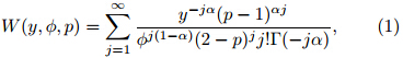
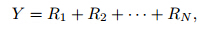
The Tweedie density function has no closed formexcept for some special cases. Numerical methods areneeded to evaluate the infinite series in Eq.(1). Figure 1 shows the density functions of some Tweedie distributionsfor 1 < p < 2. In addition to the continuousdistribution for Y > 0, there is also a point mass ofprobability at Y = 0 for each Tweedie distribution.
 |
| Fig. 1. Some Tweedie density functions for 1< p <2. Geometricsymbols indicate the point masses of probabilityat Y = 0. In each case, the mean and variance are fixed at1 and 3, respectively. |
GAMs are semi-parametric extensions of GLMs.Like a GLM, a GAM uses a link function to establisha relationship between the mean of the responsevariable Y having a distribution from the exponentialfamily and additive smooth functions of explanatoryvariables x1, x2, . . ., xp, as follows:
where μ = E[Y ], g(·) is a smooth monotonic link function, β0 is a constant, and various forms of s(·)aresmooth functions of explanatory variables. It is possible to build this kind of model structures withinthe GLM framework using polynomials or orthogonalbases to represent nonlinearities, e.g., using Legendrepolynomials to represent regional effects and Fourier series to represent seasonal cycles(Chandler and Wheater, 2002; Yang et al., 2005). However, suchan approach has two main problems: model selectionis rather cumbersome and the basis selected can havea strong influence on the fitted model. In the GAMframework, one efficient approach to implement themodel is using penalized regression splines to representthe smooth terms(Wood and Augustin, 2002).The smooth functions are rewritten using a set of basisfunctions, each of which has an associated penaltythat controls its effective degrees of freedom through asingle smoothing parameter that can be determined byminimizing some objective functions. For a comprehensiveintroduction to this approach, refer to Wood(2006).
Usually, the spatial variation of precipitation overan area can be represented as a function of a twodimensionalvector variable x with its two componentsbeing longitude and latitude or projected x-y coordinates.In GAM, the smooth function s(x) can be implementedusing thin plate regression splines(Wood, 2003). Seasonal cycles and longer-term time effectscan be represented by one-dimensional smooth functions.Time consistencies of precipitation can be representedby introducing some auto-regression terms. Inaddition, large-scale external forcings on local precipitationcan also be introduced linearly or nonlinearly.The Tweedie distribution itself is a member of the exponentialfamily. Therefore, it is possible to buildcomprehensive spatial-temporal precipitation modelsby fitting a single distribution to a set of multi-site observationsfor a certain period in the GAM frameworkfor various purposes. Here, GAMs are used to forecastprecipitation conditional on an ensemble memberindividually.2.3 BMA
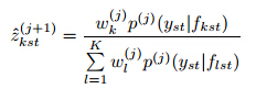
For ensemble probabilistic forecasting, BMA is astatistical technique that combines inferences and predictionsbased on individual ensemble members, so asto yield a more skillful and reliable probabilistic prediction.Assume that the forecast PDF of a weathervariable y conditional on the ensemble member forecastfk is pk(y|fk), the BMA forecast PDF is then
where wk is the posterior probability of forecast k, beingthe best one given the observations in the trainingperiod and subject to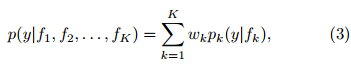
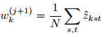
 . The BMA ensembleforecast is essentially an average of forecasts basedon individual members weighted by the likelihood thatan individual forecasting model is correct given the observations.Denote
  then the posterior mean and variance of BMA forecastcan be expressed as
Equation(3)is a finite mixture density(McLachlan and Peel, 2000)with a general form of
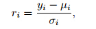
Residual diagnostics is an effective way to assessfitted models. Here Pearson residuals are used to checkthe systematic structure captured by a model. ThePearson residual for the ith observation yi is defined as
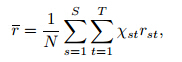
 . Then100(1–α)% limits for this mean are approximately at±Zα/2s.e.(r), where Zα/2 is the st and ard normal upperquantile at α/2 and s.e.(r)is the st and ard errorof the mean residual. For a spatial-temporal precipitationmodel, by introducing appropriate covariatesrepresenting auto-regressions, residuals from the fittedmodel can be thought of as temporally independent.However, without the spatial dependence considered, they may still be dependent spatially unless all thesites are far enough from each other. The variancefor the mean of residuals independent temporally butdependent spatially can be estimated by
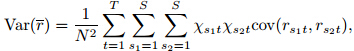
The mean residuals can be computed over subsetsby site or by time. If the fitted model is correct, the mean residuals should not show significant trends and about 100(1–α)% of them should be within thecorresponding limits. Otherwise, there might be someunexplained structures that should be taken into accountby the model.2.5 Forecast verification
Three widely used scoring rules, the mean absoluteerror(MAE), the continuous ranked probabilityscore(CRPS), and the Brier score(BS)(Jolliffe and Stephenson, 2003), are considered here to verify theBMA probabilistic forecasts. The MAE is defined as
 is the deterministic forecastgiven by the median of the forecast PDF, and Nis the number of test data.
The CRPS is defined as
The BS for probability forecasts of K complete and mutually exclusive categories is given by
 is the forecasted probability of the kth categorysubject to
 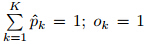 if the event occurs and 0 otherwise such that there are K−1 zeros and a single 1 contained in ok, k = 1, . . ., K; nk isthe number of observations for the kth category and nk × K = N. The BS is essentially the mean squarederror of the probability forecasts.
All these three scoring rules are negatively oriented, i.e., the smaller the values, the better the forecasts.The BS takes on values only in the range [0, 1].2.6 Computational implementation
Although the methods described above involvecomplicated computations, in the R environment(R Development Core Team, 2011), these can be easilyimplemented without heavy coding. The GAMs arefitted using the package “mgcv”(Wood, 2006). TheTweedie family of distributions is computed using thepackage “tweedie”(Dunn, 2009). Functions for numericalintegration and optimization are also availablein R.
In the fitting of each component of the BMAforecast PDF in Eq.(3)using the Tweedie familyGAMs, the power p is the parameter that determineswhich Tweedie distribution is used and should be specifiedprior to the fitting. The mean μ is expressedby smooth functions of covariates and the dispersionφ is assumed to be constant. These two parametersare member-specific and can be estimated by the individualfitting. The power p can be assumed to bea constant for all the component PDFs in Eq.(3)sothat except for weights w there is only one additionalparameter p in the mixture density function. Parametersp and w can be estimated by maximizing thelog-likelihood of the mixture density for the trainingdata using the EM algorithm described in Subsection2.3. The parameter p is estimated numerically by optimizingthe log-likelihood function using the currentestimations of w at each M step. However, when practicedin the example given in the next section, thisprocedure showed so slow a convergence rate that itis actually impractical for operations. An alternativeto this is searching p for the maximum log-likelihoodof each component PDF in Eq.(3)individually sothat all the three parameters of the Tweedie family ofdistributions are member-specific and only w are estimatedby the EM iteration. This procedure was muchfaster than the former one while the same maximumlog-likelihood was reached. The estimated wk differedonly slightly from the former results. The exampleBMA model described in the next section was finallyfitted using this procedure.3. Example results3.1 Data description and model fitting
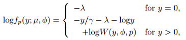
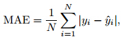
The BMA probabilistic precipitation forecastingwas applied to daily 24-h forecasts of 24-h accumulatedprecipitation over the Yishusi River basin in NorthChina throughout July 2007. The Yishusi River consistsof three main branches, namely, Yi River, ShuRiver, and Si River. It starts from Yimeng Mountainin Sh and ong Province and runs into the YellowSea crossing Henan, Anhui, and Jiangsu provinces.The total area of the basin is about 7.96×10⁴ km2.Example stations in the basin are shown in Fig. 2, 40 of which are training stations(triangles) and theother 4 test stations(dots). Precipitation data fromthese stations were provided by the China MeteorologicalAdministration. There were several rainstormsthat occurred over the basin in that month; the highestrecorded 24-h accumulated precipitation was 259.6mm at Shouxian station on the 8th. Contours in Fig. 2 show the averaged 24-h precipitation over the month.The 21-member 1°×1° NCEP ensemble precipitationforecasts retrieved from TIGGE were interpolated atthese stations as ensemble forecasts corresponding tothe observations.
 |
| Fig. 2. Example stations in the Yishusi River basin. Triangles represent training stations and dots represent teststations. Contours show the averaged 24-h precipitation(mm)over July 2007. |
Sloughter et al.(2007)found out the optimizedlength of training period by minimizing the MAE orCRPS. They concluded through their examples that30 days was enough and that longer period would notsignificantly reduce the scores. For the study area wechose, these scores are sensitive to the length of thetraining period, because over the East Asian monsoonregion where the river basin is located, the seasonalvariability of precipitation is very significant. Nevertheless, 30 days is still a proper length of time periodduring which the precipitation is approximately homogeneousfor the study area. If the training periodis long and the precipitation is inhomogeneous temporally, the model should include explicitly some covariatesrepresenting seasonality or even longer-timeeffects. Since here we intend to give an illustrativeexample rather than a complicated “perfect” solution, we take 30 days as the length of the training periodduring which we assume that the precipitation is homogeneousin time.
Exploratory analysis shows that the observationalseries at each station has high correlations with correspondingforecast series at lags from 0 to 2 days, withthe lagged correlations even higher than its autocorrelations.By taking all these considerations together, the precipitation forecast model using GAMs based onthe kth member of the ensemble forecast is constructedas
where μi(k)(t) is the mean of the Tweedie distributionof precipitation at the ith station on day t conditionalon the kth member of the ensemble forecast, xi is thetwo-dimensional coordinates of the ith station, fi(k)(t)is the kth member of the ensemble forecast for theith station on day t, and s represents one- or twodimensionalsmoothing regression splines. To achievea better fit, the cubic roots of the ensemble forecastsrather than the original values are taken in the modelfitting, just as treated in Sloughter et al.(2007) and many other works.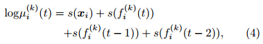
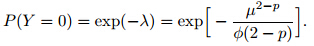
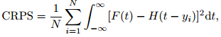
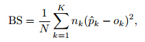
After all the individual models are fitted, the resultedforecast PDFs are then properly weighted and summed up to produce the final BMA forecast PDF.Figure 3 shows the weights estimated using the EM algorithmfor the 21 components fitted to the period of1–30 July 2007. It can be seen that except for 5 components, all the other weights are almost cut down to0. Figure 4 shows the mean Pearson residuals(circles)of the fitted BMA forecast model by site(Fig. 4a) and by day(Fig. 4b). Lines show the 95% confidencelimits. There is an apparent outlier from Dingtao stationon the 11th. The recorded precipitation for thatday was 54.6 mm; however, not only all the ensemblemembers forecasted an amount of 0 for that day, butboth the ensemble forecast and recordings for the previous3 days were all 0s as well. This case exceptionallyviolated the relationship assumed in the model specifiedby Eq.(4) and resulted in the Pearson residualfor that day as high as 22.3, and this is reflected onthe mean residual plots. Except for this case, and fora little bit overestimation for a few stations, the systematicspatial and temporal patterns of precipitationwere well captured by the BMA forecast model.
 |
| Fig. 3. Estimated weights for the 21 BMA componentsfitted to the period of 1–30 July 2007. The first 20 are forcomponents conditional on perturbed runs of the ensembleforecast and the last one on the control run. |
 |
| Fig. 4. Mean Pearson residuals(circles)of the fitted BMA forecast model by site(a) and by day(b). Lines show the95% confidence limits, which are adjusted for spatial dependence between sites. |
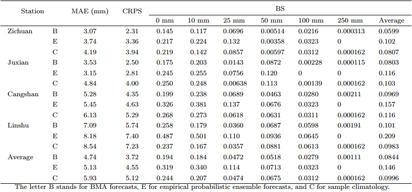
The dynamic BMA forecasting for the 4 test stationsproceeded through July 2007 using a slidingtraining period of 30 days. Empirical PDFs of theraw ensemble forecasts and the sample climatologywere also used respectively to generate forecastsfor comparison. Table 1 shows the MAE, CRPS, and BS of BMA forecasts, empirical probabilistic ensembleforecasts, and sample climatology for each station and their averages over the four stations. It can beseen that the BMA forecasts outperformed the othertwo in almost every category under comparison.
 |
To early warnings of floods, what is more importantis the forecast for extreme precipitation that canresult in floods. Among the 120 records from the 4test stations, the top 10% of them can be regardedas extreme events for the period of interest, and 4 ofwhich are greater than 50 mm. Figure 5 shows theBMA 50th(solid lines) and 90th(dashed lines)percentileforecasts compared with observations(circles)for the 4 test stations through July 2007. Figure 6 isthe counterpart of Fig. 5 for empirical probabilisticensemble forecasts. If we take the medians as the deterministicforecasts, although the BMA deterministicforecasts for heavy precipitation are smaller than theobservations in general, almost all the BMA 90th percentileupper bounds exceed the observations(thereis only one apparent exception). In contrast, almostall the corresponding upper bounds forecasted by theempirical ensemble PDFs are below the heavy rainfallobservations. Have in mind that except for spatial coordinates and ensemble forecasts, no other informationon the test stations was considered in the BMA forecasting, the BMA results are really impressive. Thiscomparison also indicates that the BMA forecasts aremuch better calibrated than the empirical probabilisticensemble forecasts.
 |
| Fig. 5. The BMA 50th(solid lines) and 90th(dashed lines)percentile forecasts of 24-h precipitation and the observations(circles)for the 4 test stations through July 2007. |
 |
| Fig. 6. The counterpart of Fig. 5 for the empirical probabilistic ensemble forecasts. |
In this paper, we proposed a BMA probabilisticprecipitation forecasting model. GAMs were used tofit the spatial-temporal precipitation models to individualensemble member forecasts. The distributionsof the precipitation occurrence and the cumulative precipitationamount were represented simultaneously bya single Tweedie distribution. BMA was then used tomix up the GAMs and to yield the final mixture model.The mixing weights were estimated using the EM algorithmmaximizing the log-likelihood of the mixturemodel. The residual diagnostics was used to examineif the fitted BMA forecasting model had fully capturedthe spatial and temporal patterns of precipitation forthe study area and the period of interest. The wholeprocedure was applied to an example dataset from theYishusi River basin for July 2007 using the NCEPensemble forecasts to generate the BMA probabilisticforecasts. The results were verified by applying threescoring rules and it is concluded that the BMAforecasts outperformed the empirical probabilistic ensembleforecasts particularly for extreme precipitationevents.
The reason why the BMA probabilistic forecastscaptured the extreme precipitation so well as shown inthe example is that, within the GAM framework, thenonlinear relationship between the mean of the precipitationdistribution and the covariates can be represented“as is” by the model described by Eq.(2).For highly skewed data like precipitation records, theirvariance is usually proportional to their mean, justlike samples from the gamma distribution. Once themeans for extreme precipitation events are underestimated, their variances are also underestimated. Thisis usually the case in GLMs in which the right-h and side of Eq.(2)is instead a linear combination of covariatesthat can be biased easily by the large amountof small-value events. Consequently, the forecastedupper bounds for extreme events are also underestimated.In GAMs, the additive smooth functions in Eq.(2)can represent unbiased relationships between themean and the covariates for both the small-value and extreme precipitation events, which guarantees sufficientvariances for extreme precipitation events and large enough forecasted upper bounds as well.
In the fitting of spatial-temporal precipitationmodel using GAMs, spatial independence betweensites conditional on the fitted surface was assumed.Only in the model diagnosis, adjustment was made forspatial dependence for the estimation of confidencelimits of the mean Pearson residuals. This is not aproblem in using the model for forecasting, since thesystematic spatial variation has already been incorporatedinto the model and what is needed is only themarginal forecast distribution for each station. However, when the model is used for multi-site simulationof precipitation, it is necessary to allow for spatial dependencein the model to generate realistic scenarios.One approach to implement this is the generalized additivemixed-effect models(GAMMs)(e.g., Ruppert et al., 2003), in which spatial correlation structures canbe specified. However, the incorporation of spatial correlationstructures makes the computation of GAMMsintensive and much slower than that of GAMs. Thewhole BMA post-processing procedure to incorporatespatial dependence suitable for operations needs to beworked out ad hoc.
At the stage of the numerical estimation of BMAweights, weights for extreme precipitation events arestill apt to be underestimated. A possible improvementto this is to use weighted likelihood estimatorin the EM algorithm(Markatou, 2000). The weightfunction must be carefully designed such that thelog-likelihoods of models in good agreement with observationsof heavy precipitation can receive higherweights. This will be considered in our future work.
A direct application of the method proposed hereis the downscaling of multimodel GCM simulationsfor climate change scenarios with uncertainty estimation.Since for this purpose the training period couldbe decades of years, time effects at different scalessuch as seasonal, interannual, and decadal variationsshould be explicitly represented in the model. Covariatesother than spatial and temporal variables couldbe GCM outputs representing large-scale circulationpatterns that result in the local precipitation. If spatialdependence is incorporated, the model could beused to simulate the local precipitation under climatechange scenarios. A series of fine-scale precipitationfields could be generated by such simulation modelsas input to hydrological models for the assessment ofclimate change impact.
| [1] | Chandler, R. E., and H. S. Wheater, 2002: Analysis of rainfall variability using generalized linear models: a case study from the west of Ireland. Water Resource Res., 38(10), 1192–1202. |
| [2] | Coe, R., and R. D. Stern, 1982: Fitting models to daily rainfall data. J. Appl. Meteor., 21, 1024–1031. |
| [3] | Dunn, P. K., 2004: Occurrence and quantity of precipitation can be modeled simultaneously. Int. J. Climatol., 24, 1231–1239. |
| [4] | —–, 2009: Tweedie: Tweedie Exponential Family Models. R package version 2.0.2, http://CRAN.Rproject.org/package=tweedie. |
| [5] | Gneiting, T., and A. E. Raftery, 2007: Strictly proper scoring rules, prediction, and estimation. J. Am. Stat. Assoc., 102, 359–378. |
| [6] | Hastie, T. J., and R. J. Tibshirani, 1990: Generalized Additive Models. Chapman and Hall, London, 335 pp. |
| [7] | Jolliffe, I. T., and D. B. Stephenson, 2003: Forecast Verification: A Practitioner’s Guide in Atmospheric Science. Wiley and Sons, 240 pp. |
| [8] | Markatou, M., 2000: Mixture models, robustness, and the weighted likelihood methodology. Biometrics, 56(2), 483–486. |
| [9] | McLachlan, G. J., and D. Peel, 2000: Finite Mixture Models. Wiley, 419 pp. |
| [10] | —–, and T. Krishnan, 2008: The EM Algorithm and Extensions. 2nd Edition. Wiley, 359 pp. |
| [11] | McCullagh, P., and J. A. Nelder, 1989: Generalized Linear Models. 2nd Edition, Chapman and Hall, London, 532 pp. |
| [12] | Park, Y.-Y., R. Buizza, and M. Leutbecher, 2008: TIGGE: preliminary results on comparing and combining ensembles. Quart. J. Roy. Meteor. Soc., 134, 2029–2050. |
| [13] | R Development Core Team, 2011: R: A Language and Environment for Statistical Computing. R Foundation for Statistical Computing, Vienna, Austria. ISBN 3-900051-07-0, URL http://www.Rproject.org. |
| [14] | Raftery, A. E., T. Gneiting, F. Balabdaoui, et al., 2005: Using Bayesian model averaging to calibrate forecast ensembles. Mon. Wea. Rev., 133, 1155–1174. |
| [15] | Ruppert, D., M. P. Wand, and R. J. Carroll, 2003: Semiparametric Regression. Cambridge University Press, 386 pp. |
| [16] | Sloughter, J. M., A. E. Raftery, T. Gneiting, et al., 2007: Probabilistic quantitative precipitation forecasting using Bayesian model averaging. Mon. Wea. Rev., 135, 3209–3220. |
| [17] | Stern, R. D., and R. Coe, 1984: A model fitting analysis of daily rainfall data. J. Roy. Stat. Soc., 147A, 1–34. |
| [18] | Tweedie, M. C. K., 1984: An index which distinguishes between some important exponential families in statistics: Applications and new directions. Proceedings of the Indian Statistical Institute Golden Jubilee International Conference, J. K. Ghosh and J. Roy, Eds., Indian Statistical Institute, Calcutta, 579–604. |
| [19] | Wood, S. N., 2003: Thin plate regression splines. J. R. Statist. Soc. B, 65(1), 95–114. |
| [20] | —–, 2006: Generalized Additive Models: An Introduction with R. CRC/Chapman & Hall, Boca Raton, Florida, 392 pp. |
| [21] | —–, and N. H. Augustin, 2002: GAMs with integrated model selection using penalized regression splines and applications to environmental modeling. Eco. Modelling, 157, 157–177. |
| [22] | Yang, C., R. E. Chandler, V. S. Isham, et al., 2005: Spatial-temporal rainfall simulation using generalized linear models. Water Resource Res., 41(11), W11415. |
| [23] | Zhu, Y., 2005: Ensemble forecast: A new approach to uncertainty and predictability. Adv. Atmos. Sci., 22(6), 781–788. |