
Contribution Ratio of Excitation Sources to the Underwater Acoustic Radiation of the X-BOW Polar Exploration Cruise Ship
https://doi.org/10.1007/s11804-024-00457-8
-
Abstract
A finite element and boundary element model of the 100 m X-BOW polar exploration cruise ship is established. The vibrated velocity-excited force admittance matrix is calculated by frequency response analysis, and the vibrated velocity in the stern plate and main engine foundations is tested during the trial trip. Then, the excited force of the propeller and main engine is derived using the vibrated velocity and admittance matrix. Based on the excited force, the cabin-simulated vibrated velocity is compared with the tested vibrated velocity, and the tolerance is within the allowable scope in engineering. Loading the excited forces on the boundary element model, the distribution characteristics of sound level underwater are analyzed. Then, forces excited by the main engine and propeller are loaded on the model, and the contribution ratio of excitation sources to underwater acoustic radiation is analyzed. The result provides a reference for vibration assessment in the early stage and control in the late stage.Article Highlights● Aiming at the problem that the empirical method is not applicable and the theoretical method is difficult to solve, the propeller and main engine excitation force inversion method, based on finite element model and real ship test data, is proposed. This method deduces a more accurate excitation source and provides a reference for calculating the excitation force of ship vibration sources.● Based on the transfer path theory, the main excitation sources are selected and sorted according to the contribution rate of the excitation sources to underwater noise. This approach offers a reference method for controlling ship underwater noise. -
1 Introduction
The 100 m X-BOW polar exploration cruise ship is the first luxury polar exploration cruise ship in China. It has multiple pieces of equipment, large power, and complex hull structure and engine room layout. However, its structural characteristics produce structural vibration, generating serious underwater acoustic radiation and affecting the survival environment of underwater organisms. For the effective control of the underwater acoustic radiation of the cruise ship, the input excitation of the main excitation sources is needed, and the underwater acoustic radiation of its structure must be simulated and analyzed in the design stage.
Wang et al.(2020) developed an experimental model to investigate the effects of force and acoustic excitation on the vibration and underwater acoustic radiation of a stiffened conical-cylindrical shell. Meanwhile, a coupled precise transfer matrix method and wave superposition method was also proposed to analyze vibro-acoustic responses of combined shells. Gao et al. (2022) has measured the underwater vibration and acoustic radiation of a typical ribbed cylindrical shell structure under broadband excitation using the direct test method. The accuracy of the test results is verified by comparing them with those obtained by the numerical finite element (FE)/boundary element (BE) coupling method. The free vibration, forced vibration and acoustic radiation characteristics of stiffened submerged cylindrical shells are also thoroughly investigated. Su et al. (2018) investigated the influence of non-axisymmetric substructures such as propulsion system foundation and mass block on the vibroacoustic behavior of a simplified wreck by numerical methods and experiments. Axial and lateral force excitation of the propeller is considered in the analysis. Kehr and Kao (2011) investigates the sound field of a container ship radiated by a propeller and scattered by a free-surface hull. Propeller-induced pressure fluctuations at low blade rates on the hull were also calculated, and it was found that, due to the small retardation time, the pressure fluctuations at points near the propeller were similar to those obtained by the panel method satisfying Laplace's equation. Wu et al. (2019) compared the analytical solutions of field point sound pressure and acoustic radiation power of a reinforced cylindrical shell with the Abaqus calculated structure and verified that the method can be used for the acoustic radiation assessment of complex structures with interdimensional water bodies underwater. Fu et al. (2020) proposed two versions of hybrid FEM–SBM solvers to perform the acoustic radiation and propagation of shell structures in shallow-water marine environments. For axisymmetric shell structures under axisymmetric forces, the axisymmetric numerical formulation of a hybrid solver (AFEM–ASBM) reduces computational costs. For general shell structures, a fast direct solver based on the recursive skeletonization factorization is introduced into the hybrid solver (FEM–RSFSBM) to accelerate the computation of the underwater acoustic field. The effectiveness and accuracy of the proposed hybrid solvers are clearly demonstrated by several numerical examples. Zou et al. (2023) introduced a ring-stiffened cylindrical shell model to describe the main hull and the theoretical derivation process of the mixed analytical–numerical fluid–structure coupled vibration and underwater acoustic radiation calculation of underwater vehicle structure in detail. The viscoelastic material calculation model is established with ANSYS finite element software and combined with the analytical – numerical hybrid calculation method for the local damping treatment of underwater vehicle structure sound radiation calculation method. This method has the advantages of simple modeling and a small computation. Fu et al. (2023) presented an overview of the singular boundary method (SBM) and its various engineering applications; the basic concepts of the singular boundary method were first introduced, and then several additional schemes were introduced to resolve the non-uniqueness issue encountered in the SBM and enable the application of the SBM to large-scale engineering and scientific computing, nonhomogeneous partial differential equations, non-isotropic problems, and initial-boundary value problems. Some efficient techniques, such as moment condition and modified combined Helmholtz integral equation formulation, have been introduced into the SBM to enhance its performance.
The X-BOW polar exploration cruise ship is a relatively new ship type. Thus, no research has explored the characteristics of its underwater acoustic radiation. The cruise ship is generally the main mode of transportation for tourists in the Arctic and surrounding areas. It is a powerful ship type, and thus, its operation will inevitably cause underwater acoustic radiation and affect the survival of underwater organisms, particularly Arctic seabed species. Thus, a study of the underwater acoustic radiation of the X-BOW is needed. In this study, the finite element and boundary element models of the X-BOW polar exploration cruise were established, and the vibration velocity–excited force derivative matrix was derived through frequency response analysis. The simulation results of the vibration velocity of the engine room were compared with the test results, and the accuracy of the excited force was verified. The excitation sources were loaded on the boundary element model, and the characteristics of underwater acoustic radiation caused by the excitation sources of the X-BOW polar expedition cruise were analyzed. Moreover, the forces excited by the propeller and main engine were loaded separately for the analysis of the contribution rate of the two excitation sources to underwater acoustic. The aim was to provide a reference for the pre-assessment and post-control of underwater sound radiation of the X-BOW polar exploration cruise structure.
2 Calculation theory of the underwater acoustic radiation of X-BOW polar expedition cruise ship
2.1 Principle of vibroacoustic radiation calculation based on direct boundary method
When the ship is sailing in water, it must satisfy the following conditions when its external field is an ideal acoustic medium: 1) the flow field is uniform and isotropic; 2) the acoustic fluctuation process is an adiabatic process; 3) the fluid is a compressible ideal fluid; 4) the acoustic wave is a small-amplitude acoustic wave, and the fluid only makes linear deformation (He, 1981). On this basis, a finite baffle placed in the fluid is selected as the research object, as shown in Figure 1.
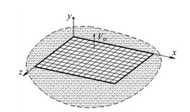 Figure 1 Finite baffle placed in the fluid
After the plate is divided into R cells (Frank and Paolo, 2006), the vertical vibration velocity of the whole plate and the sound pressure acting on each cell can be expressed as a vector group, as shown in Equations (1) and (2).
$$ \boldsymbol{v}_e=\left\{\begin{array}{llll} v_{e 1} & v_{e 1} & \cdots & v_{e R} \end{array}\right\}^{\mathrm{T}} $$ (1) $$ \boldsymbol{p}_e=\left\{\begin{array}{ll} p_{e 1} & p_{e 1} \end{array} \cdots p_{e R}\right\}^{\mathrm{T}} $$ (2) where v eR and peR represent the vertical vibration velocity of the R unit and the sound pressure acting on it, respectively. Then, the acoustic radiation power of the baffle can be expressed by Equation (3).
$$ P(\omega)=\boldsymbol{v}_e{ }^{\mathrm{H}} \boldsymbol{X} \boldsymbol{v}_e $$ (3) $$ \boldsymbol{X}=\frac{\omega^2 \rho A_e{ }^2}{4 \pi c}\left[\begin{array}{cccc} 1 & \frac{\sin \left(k L_{12}\right)}{k L_{12}} & \cdots & \frac{\sin \left(k L_{1 R}\right)}{k L_{1 R}} \\ \frac{\sin \left(k L_{21}\right)}{k L_{21}} & \frac{\sin \left(k L_{22}\right)}{k L_{22}} & \cdots & \frac{\sin \left(k L_{2 R}\right)}{k L_{2 R}} \\ \vdots & \vdots & \ddots & \vdots \\ \frac{\sin \left(k L_{R 1}\right)}{k L_{R 1}} & \frac{\sin \left(k L_{R 2}\right)}{k L_{R 2}} & \cdots & 1 \end{array}\right] $$ where Lij is the distance between the i and j cell, ρ is the fluid density, k is the wave number of the air, Ae is the radiation area, and is the propagation speed of sound waves in the fluid. Equation (3), which is based on the direct boundary method, uses the finite element concept to solve the plate vibration acoustic radiation equation. In the above equation, the vibration velocity of the plate needs to be a known input as the boundary condition for the sound field solution.
2.2 X-BOW polar exploration cruise underwater acoustic radiation model
Based on the direct boundary method, the X-BOW polar exploration cruise underwater acoustic radiation model is established (Figure 2). The size of the near sound field is 200 m×100 m×100 m, and acoustic reflection is prevented by setting up an infinite boundary in the sound field truncation. The far field can be defined according to Equation (4), that is,
$$ L>\frac{D}{\lambda} $$ (4) 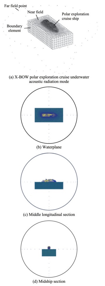 Figure 2 X-BOW polar exploration cruise underwater acoustic radiation model
where D is the length of the ship, k is the wavelength, and ρ is the distance between the receiving point and the sound source. According to Equation (4), the three planes of the far sound field points are established on the basis of the waterline plane, mid-longitudinal section, and mid-transverse section. The X-BOW polar exploration cruise finite element model is 104 m in length, 18 m in width, 5.1 m in waterline height, and 4 265 t in weight. The additional mass and center of gravity of the model strictly follow the weight center of gravity report. The grid size is 400 mm×400 mm, the plate structure is composed of quad4 and tria3 cells, and the beam structure is a bar2 cell (Figure 3).
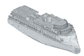 Figure 3 X-BOW polar exploration cruise finite element model
3 Calculation of excited force for X-BOW polar exploration cruise
In Equation (3), the magnitude of the main excited source needs to be obtained first so that the vibration velocity of the structure can be solved as the boundary condition for the underwater acoustic radiation analysis. The excited force is solved mainly with the traditional transfer path analysis principle, which is applicable to linear and timeinvariant systems (Cinkraut, 2016). The main principle is illustrated in Figure 4, where Fn is the nth input force, Dn is the admittance of the nth transfer path, and the total response of the observation point is the sum of the response contributions on each transfer path.The response contribution on each transfer path is the product of the excited force and the admittance of the transmission path.
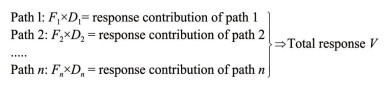 Figure 4 Transmission pathway analysis schematic
When Fn is assumed to be the excited force of the vibration source of the cruise ship, Vm is the vibration velocity response of the observation point, and Dnm is the admittance of the transmission path from the excitation point n to the observation point m. Equation (5) can be obtained.
$$ \left\{\begin{array}{c} V_1 \\ V_2 \\ \vdots \\ V_m \end{array}\right\}=\left[\begin{array}{cccc} D_{11} & D_{21} & \cdots & D_{n 1} \\ D_{12} & D_{22} & \cdots & D_{n 2} \\ \vdots & \vdots & \ddots & \vdots \\ D_{1 m} & D_{2 m} & \cdots & D_{n m} \end{array}\right]\left\{\begin{array}{c} F_1 \\ F_2 \\ \vdots \\ F_m \end{array}\right\} $$ (5) If vm and Dnm are known, the above equation is multiplied left and right simultaneously by the inverse matrix of the admittance matrix for the derivation of Equation (6).
$$ \left[\begin{array}{cccc} D_{11} & D_{21} & \cdots & D_{n 1} \\ D_{12} & D_{22} & \cdots & D_{n 2} \\ \vdots & \vdots & \ddots & \vdots \\ D_{1 m} & D_{2 m} & \cdots & D_{n m} \end{array}\right]^{-1}\left\{\begin{array}{c} V_1 \\ V_2 \\ \vdots \\ V_m \end{array}\right\}=\left\{\begin{array}{c} F_1 \\ F_2 \\ \vdots \\ F_n \end{array}\right\} $$ (6) To ensure that the equation has a solution, we assume that the admittance matrix is an order matrix. Then, the excited force can be obtained.
3.1 Excitation main frequency analysis of X-BOW polar expedition cruise
The main causes of the steady-state forced vibration of the ship are the unbalanced inertia force of the reciprocating machine on board and the disturbance force caused by the propeller and the air bubble near the high-speed ship (Jin and Xia, 2011). When the cruise ship is sailing at high speed, a large number of air bubbles are generated on the propeller blades, and the pulsation pressure generated by the propeller blades on the bottom of the ship is considerable (Hajime, 1976). Previous real ship tests consider the surface force induced by the propeller as the most important factor among the propeller vibration sources (He, 1981). Therefore, the excitation source in this paper only considers the excited force of the main engine and surface pulse power caused by the propeller.
The X-BOW polar exploration cruise adopts two propellers and two rudders, the propeller diameter is 3 100 mm, the 80% rated working speed is 192 r/min, and the propeller excitation blade frequency can be calculated by Equation (7).
$$ f=\frac{n \times Z}{60} $$ (7) where n is the speed and Z is the number of propeller blades. The ship uses a four-blade propeller, and thus, the propeller pulsation excitation blade frequency is 12.8 Hz.
The main engine firing frequency can be obtained
$$ f=\frac{n Z}{60} m $$ (8) where n is the rotational speed, Z is the number of cylinders, and the four-stroke diesel engine m is 0.5. X-BOW polar expedition cruise has two kinds of four-stroke main engines, where the numbers of cylinders are 8 and 6, and 80% of the rated working speed is 1 000 r/min. From Equation (8), it can be known that the firing frequencies of the two main engines are 66.8 and 50 Hz.
The base frequency of the main engine can be calculated using Equation (9).
$$ f=\frac{n}{60} $$ (9) The fundamental frequency of both main engines is 16.7 Hz.
3.2 Propeller pulsation excitation
For the calculation of the propeller pulsation excitation, the vibration velocity and transmission path guide should be obtained. During the sea trial of the X-BOW polar exploration cruise, the stern bottom plate directly above the propeller is selected as the test object, and six measurement points are arranged for the measurement of the vibration velocity of the ship bottom plate directly above the propeller under 80% sailing conditions through the test (Figure 5); Vn is denoted by the vibration velocity of measurement point n, n = 1, 2, …, 6.
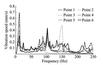 Figure 5 Vibration velocity of the ship bottom plate directly above the propeller
The propeller pulsation excitation is a nonuniformly distributed pressure field. Thus, determining the propeller pulsation excitation area first is necessary, and a practical method is to select the area above the propeller as the propeller pulsation excitation area within an area with propeller diameter D squared (Det, 1983) (Figure 6). Given that the propeller pulsation excitation is a nonuniformly distributed pressure field, a simplified method is needed to simulate the nonuniformly distributed pressure field. The port and starboard propeller pulsation excitation regions are divided into six force regions, which jointly carry the nonuniformly distributed pressure field of the propeller, and each force region is a uniformly distributed pressure field. The surface force in the nth force area is denoted by Fn (Figure 7).
 Figure 6 Propeller pulsation excitation area map
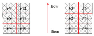 Figure 7 Propeller pulsation excited force area division
To obtain the transfer path conductance from each force area to each observation area, we make Fn (n = 1, 2, …, 12) equal to 1N in the full frequency band and load on each force area of the cruise finite element model. Then, the transfer path conductance is obtained by conducting a frequency response analysis on each observation point. Figure 8 shows the conductance curve from each propeller excited force area to measurement point 1 on the starboard side. The comparison between Figures 5 and 8 shows that the conduction curves are flat at 12.5 and 25 Hz without resonance peaks, and the fundamental frequency of the host excitation is 16.7 Hz, which has no excitation contribution to these two frequency points. Thus, the wave peak frequencies at the low frequency of vibration speeds of 12.5 and 25 Hz correspond to the lobe frequency and times lobe frequency of the propeller pulsation excitation. In the conduction curves near 100–150 Hz, an obvious resonant wave peak appears. The wave peak frequency of vibration velocity near 100–150 Hz corresponds to the resonant frequency of the local structure of the ship bottom.
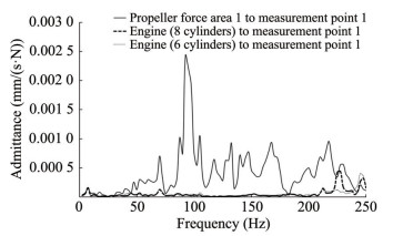 Figure 8 Transfer path admittance of each propeller excited force area on the starboard side to measurement point 1
Owing to the presence of the main engine–excited force, whether the main engine–excited force has an effect on the vibration velocity of the observation point should be considered. The nearest excitation point on the base of the host is selected, and the unit force of the full frequency band is loaded on the excitation point for frequency response analysis and calculation of the transfer path admittance. Figure 9 shows the comparison of the transfer path admittance from the main engine excitation point and the propeller excitation point 1 to the observation point 1. Therefore, when the propeller pulsation excitation is back-propelled, the contribution of the host excitation to the velocity of the measurement point can be ignored. Substituting the transfer path conductance Dn, m and the measurement point velocity Vn into Equation (5), we get
$$ \begin{aligned} \left\{\begin{array}{c} V_1 \\ V_2 \\ \vdots \\ V_6 \end{array}\right\} & =\left[\begin{array}{cccc} D_{1, 1} & D_{2, 1} & \cdots & D_{6, 1} \\ D_{1, 2} & D_{2, 2} & \cdots & D_{6, 2} \\ \vdots & \vdots & \ddots & \vdots \\ D_{1, 6} & D_{2, 6} & \cdots & D_{6, 6} \end{array}\right]\left\{\begin{array}{c} F_1 \\ F_2 \\ \vdots \\ F_6 \end{array}\right\} \\ & +\left[\begin{array}{cccc} D_{7, 1} & D_{8, 1} & \cdots & D_{12, 1} \\ D_{7, 2} & D_{8, 2} & \cdots & D_{12, 2} \\ \vdots & \vdots & \ddots & \vdots \\ D_{7, 6} & D_{8, 6} & \cdots & D_{12, 6} \end{array}\right]\left\{\begin{array}{c} F_7 \\ F_8 \\ \vdots \\ F_{12} \end{array}\right\} \end{aligned} $$ (10) 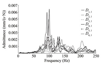 Figure 9 Comparison of transfer path admittance from excitation source to measurement point 1
Given that the two propellers are antisymmetric, the surface force should also be antisymmetric, that is,
$$ \left\{\begin{array}{lll} F_1=F_7 & F_2=F_8 & F_3=F_9 \\ F_4=F_{10} & F_5=F_{11} & F_6=F_{12} \end{array}\right. $$ (11) Thus Equation (10) can be converted to:
$$ \left\{\begin{array}{c} V_1 \\ V_2 \\ \vdots \\ V_6 \end{array}\right\}=\left[\begin{array}{cccc} D_{1, 1}+D_{7, 1} & D_{2, 1}+D_{8, 1} & \cdots & D_{6, 1}+D_{12, 1} \\ D_{1, 2}+D_{7, 2} & D_{2, 2}+D_{8, 2} & \cdots & D_{6, 2}+D_{12, 2} \\ \vdots & \vdots & \ddots & \vdots \\ D_{1, 6}+D_{7, 6} & D_{2, 6}+D_{8, 6} & \cdots & D_{6, 6}+D_{12, 6} \end{array}\right]\left\{\begin{array}{c} F_1 \\ F_2 \\ \vdots \\ F_6 \end{array}\right\} $$ (12) Multiplying the inverse matrix of the admittance matrix to the left and right of Equation (12) simultaneously results in
$$ \left[\begin{array}{cccc} D_{1, 1}+D_{7, 1} & D_{2, 1}+D_{8, 1} & \cdots & D_{6, 1}+D_{12, 1} \\ D_{1, 2}+D_{7, 2} & D_{2, 2}+D_{8, 2} & \cdots & D_{6, 2}+D_{12, 2} \\ \vdots & \vdots & \ddots & \vdots \\ D_{1, 6}+D_{7, 6} & D_{2, 6}+D_{8, 6} & \cdots & D_{6, 6}+D_{12, 6} \end{array}\right]^{-1}\left\{\begin{array}{c} V_1 \\ V_2 \\ \vdots \\ V_6 \end{array}\right\}=\left\{\begin{array}{c} F_1 \\ F_2 \\ \vdots \\ F_6 \end{array}\right\} $$ (13) The above equation is solved by Matlab, and the final propeller pulsation excited force can be obtained, as shown in Figure 10, which shows that the propeller pulsation excited force is mainly distributed around the half-blade frequency (7 Hz), blade frequency (12.5 Hz), and multiblade frequency (25 Hz). The most evident force is observed at the blade frequency.
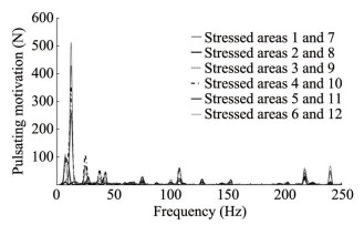 Figure 10 Propeller pulsation excitation
3.3 Main engine motivation
Four four-stroke main engines are installed in the X-BOW polar exploration cruise. Main engines A and C are Wärtsilä 8L20 with a maximum power of 1 600 kW and eight cylinders. Main engines B and D are Wärtsilä 6L20 with a maximum power of 1 200 kW, six cylinders, and a rated speed of 1 000 r/min (Figure 11). As demonstrated in Equation (8), the firing frequency of main engines A and C is 66.8 Hz, and the firing frequency of main engines B and D is 50 Hz.
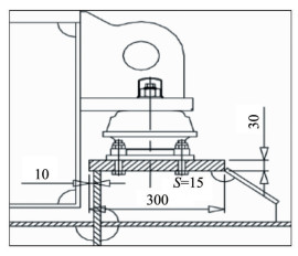 Figure 11 Schematic diagram of main engine vibration isolator installation
The measurement points are arranged and numbered at the bolted connection between the mainframe and base. The finite element model of the mainframe base and the numbering arrangement of the measurement points are shown in Figure 12. The vibration velocity is measured at measurement point 1 (Figure 13). The five main waveform frequencies of the vibration velocity of the main measurement point 1 are 12.5, 17.5, 25, 50 and 67.5 Hz, which correspond to the blade frequency of the propeller pulsation excitation, the fundamental frequency of the main engine, the octave frequency of the propeller pulsation excitation, and the firing frequency of the two main engines. Therefore, the contribution of the propeller pulsation excitation to the vibration velocity of each measurement point and the interaction between the main engines need to be considered in the calculation of the main engine–excited force.
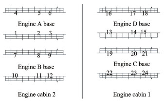 Figure 12 Finite element model of mainframe base and measurement point arrangement
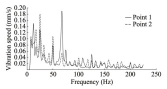 Figure 13 Vibration velocity of measurement point 1 and measurement point 7
To verify the mutual influence between the main engine excitation, we apply the full-band unit force to each foot on the main engine base. The conductance of each transfer path is obtained through frequency response analysis. The base measurement point 1 in the main compartment 2 of main engine A is investigated. First, the influence of the adjacent compartment base is analyzed (Figure 14) for the transfer path admittance from measurement points 1, 13, and 19 to measurement point 1. The transfer path admittance from the site between the base measurement points 13 and 19 to measurement point 1 is much smaller than the measurement point 1 origin admittance, and thus, the main engine excitation contribution in compartment 1 can be ignored during the back-propagation of the main engine– excited force in compartment 2 in the main engine base. Using measurement point 1, we analyze the interaction of the excitation of each measurement point in main cabin 2 (Figure 15) for the transfer path admittance from measurement points 1–3, 4, 7–9, and 10 to measurement point 1. The transfer path admittance from measurement points 4 and 10 to measurement point 1 is much smaller than the transfer path admittance from other measurement points to measurement point 1. Meanwhile, given that measurement points 5, 6, 11, and 12 are far from measurement point 1, the excitation contribution of measurement points 4–6 and 10–12 to measurement point 1 can be neglected. The same conclusion can be obtained from the analysis of measurement points 2 and 3. Therefore, in the back-projection of the excited force in points 1–3 and 7–9, the excitation contribution of points 4–6 and 10–12 can be ignored, but the self-excitation contribution of points 1–3 and 7–9 and the propeller pulsation excitation contribution should be considered. When the excited force of points 4–6 is backprojected, only the propeller pulsation excitation contribution and the self-excitation contribution of points 4–6 should be considered.
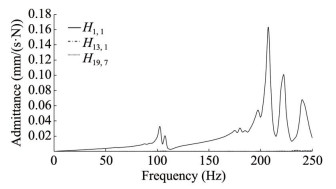 Figure 14 Transfer path admittance from measurement points 1, 13, and 19 to measurement point 1
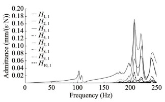 Figure 15 Transfer path admittance from measurement points 1 to 3, 4, 7–9, and 10 to measurement point 1
The variable Un denotes the vibration velocity at the foot of the base, Tn denotes the vertical excitation at the foot, Mmn denotes the transfer path admittance from the propeller pulsation excitation region to the host base, and Hmn denotes the transfer path admittance between the host bases. Equation (14) is as follows:
$$ \left\{\begin{array}{l} U_1 \\ U_2 \\ U_3 \\ U_7 \\ U_8 \\ U_9 \end{array}\right\}=\left[\begin{array}{llll} M_{1, 1}+M_{7, 1} & M_{2, 1}+M_{8, 1} & \cdots & M_{6, 1}+M_{12, 1} \\ M_{1, 2}+M_{7, 2} & M_{2, 2}+M_{8, 2} & \cdots & M_{6, 2}+M_{12, 2} \\ M_{1, 3}+M_{7, 3} & M_{2, 3}+M_{2, 3} & \cdots & M_{12, 3}+M_{12, 3} \\ M_{1, 7}+M_{7, 7} & M_{2, 7}+M_{2, 7} & \cdots & M_{12, 7}+M_{12, 7} \\ M_{1, 8}+M_{7, 8} & M_{2, 8}+M_{2, 8} & \cdots & M_{12, 8}+M_{12, 8} \\ M_{1, 9}+D_{7, 9} & M_{1, 9}+M_{7, 9} & \cdots & M_{12, 9}+M_{12, 9} \end{array}\right]\left\{\begin{array}{c} F_1 \\ F_2 \\ \vdots \\ F_6 \end{array}\right\}+\left[\begin{array}{llllll} H_{1, 1} & H_{2, 1} & H_{3, 1} & H_{7, 1} & H_{8, 1} & H_{9, 1} \\ H_{1, 2} & H_{2, 2} & H_{3, 2} & H_{7, 2} & H_{8, 2} & H_{9, 2} \\ H_{1, 3} & H_{2, 3} & H_{3, 3} & H_{7, 3} & H_{8, 3} & H_{9, 3} \\ H_{1, 7} & H_{2, 7} & H_{3, 7} & H_{7, 7} & H_{8, 7} & H_{9, 7} \\ H_{1, 8} & H_{2, 8} & H_{3, 8} & H_{7, 8} & H_{8, 8} & H_{9, 8} \\ H_{1, 9} & H_{2, 9} & H_{3, 9} & H_{7, 9} & H_{8, 9} & H_{9, 9} \end{array}\right]\left\{\begin{array}{l} T_1 \\ T_2 \\ T_3 \\ T_7 \\ T_8 \\ T_9 \end{array}\right\} $$ (14) The excited force at points 1, 2, 3, 7, 8, and 9 can be calculated from the above equation as
$$ \left[\begin{array}{llllll} H_{1, 1} & H_{2, 1} & H_{3, 1} & H_{7, 1} & H_{8, 1} & H_{9, 1} \\ H_{1, 2} & H_{2, 2} & H_{3, 2} & H_{7, 2} & H_{8, 2} & H_{9, 2} \\ H_{1, 3} & H_{2, 3} & H_{3, 3} & H_{7, 3} & H_{8, 3} & H_{9, 3} \\ H_{1, 7} & H_{2, 7} & H_{3, 7} & H_{7, 7} & H_{8, 7} & H_{9, 7} \\ H_{1, 8} & H_{2, 8} & H_{3, 8} & H_{7, 8} & H_{8, 8} & H_{9, 8} \\ H_{1, 9} & H_{2, 9} & H_{3, 9} & H_{7, 9} & H_{8, 9} & H_{9, 9} \end{array}\right]^{-1}\left\{\begin{array}{c} U_1 \\ U_2 \\ U_3 \\ U_7 \\ U_8 \\ U_9 \end{array}\right\}-\left[\begin{array}{llll} M_{1, 1}+M_{7, 1} & M_{2, 1}+M_{8, 1} & \cdots & M_{6, 1}+M_{12, 1} \\ M_{1, 2}+M_{7, 2} & M_{2, 2}+M_{8, 2} & \cdots & M_{6, 2}+M_{12, 2} \\ M_{1, 3}+M_{7, 3} & M_{2, 3}+M_{2, 3} & \cdots & M_{12, 3}+M_{12, 3} \\ M_{1, 7}+M_{7, 7} & M_{2, 7}+M_{2, 7} & \cdots & M_{12, 7}+M_{12, 7} \\ M_{1, 8}+M_{7, 8} & M_{2, 8}+M_{2, 8} & \cdots & M_{12, 8}+M_{12, 8} \\ M_{1, 9}+M_{7, 9} & M_{1, 9}+M_{7, 9} & \cdots & M_{12, 9}+M_{12, 9} \end{array}\right]\left\{\begin{array}{l} F_1 \\ F_2 \\ \vdots \\ F_6 \end{array}\right\}=\left\{\begin{array}{l} T_1 \\ T_2 \\ T_3 \\ T_7 \\ T_8 \\ T_9 \end{array}\right\} $$ (15) The excited forces at points 4, 5, 6, 10, 11, and 12 are
$$ \left.\left[\begin{array}{ccc} H_{4, 4} & H_{5, 4} & H_{6, 4} \\ H_{4, 5} & H_{5, 5} & H_{6, 5} \\ H_{4, 6} & H_{5, 6} & H_{6, 6} \end{array}\right]^{-1}\left\{\begin{array}{c} U_4 \\ U_5 \\ U_6 \end{array}\right\}-\left[\begin{array}{cccc} M_{1, 4}+M_{7, 4} & M_{2, 4}+M_{8, 4} & \cdots & M_{6, 4}+M_{12, 4} \\ M_{1, 5}+M_{7, 5} & M_{2, 5}+M_{8, 5} & \cdots & M_{6, 5}+M_{12, 5} \\ M_{1, 6}+M_{7, 6} & M_{1, 6}+M_{7, 6} & \cdots & M_{6, 6}+M_{12, 6} \end{array}\right]\left\{\begin{array}{c} F_1 \\ F_2 \\ \vdots \\ F_6 \end{array}\right\} \right\rvert\, =\left\{\begin{array}{c} T_4 \\ T_5 \\ T_6 \end{array}\right\} $$ (16) $$ \left[\begin{array}{ccc} H_{10, 10} & H_{11, 10} & H_{12, 10} \\ H_{10, 11} & H_{11, 11} & H_{12, 11} \\ H_{10, 12} & H_{11, 12} & H_{12, 12} \end{array}\right]^{-1}\left\{\left\{\begin{array}{c} U_{10} \\ U_{11} \\ U_{12} \end{array}\right\}-\left[\begin{array}{llll} D_{1, 10}+D_{7, 10} & D_{2, 10}+D_{8, 10} & \cdots & D_{6, 10}+D_{12, 10} \\ D_{1, 11}+D_{7, 11} & D_{2, 11}+D_{8, 11} & \cdots & D_{6, 11}+D_{12, 11} \\ D_{1, 12}+D_{7, 12} & D_{1, 12}+D_{7, 12} & \cdots & D_{6, 12}+D_{12, 12} \end{array}\right]\left\{\begin{array}{c} F_1 \\ F_2 \\ \vdots \\ F_6 \end{array}\right\}=\left\{\begin{array}{c} T_{10} \\ T_{11} \\ T_{12} \end{array}\right\}\right. $$ (17) To simplify the process, the following equations are used.
$$ T_{\mathrm{AC}}=\frac{\sqrt{\sum\left(T_n\right)^2}}{6} n=1, 2, \cdots, 6 $$ (18) $$ T_{\mathrm{BD}}=\frac{\sqrt{\sum\left(T_m\right)^2}}{6} m=7, 8, \cdots, 12 $$ (19) The variable TAC is the excited force of hosts A and C, and TBD is the excited force of hosts B and D. The spectra of TAC and TBD are shown in Figure 17.
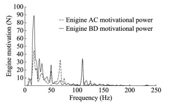 Figure 16 Main engine–excited force
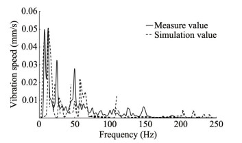 Figure 17 Second-deck laundry room
3.4 Excited force validation
To verify the accuracy of the excited force, we apply the propeller pulsation excited force and the main engine excitation to the finite element model for spectral analysis. The four areas close to the excitation source are selected: the second-deck laundry room, second-deck crew room, thirddeck stern storage room, and fourth-deck passenger compartment. The simulation analysis results of these areas are compared with the test results (Figures 17‒20). The simulation and test curves change in the same manner. The effective value of vibration speed is compared (Table 1). The maximum error is 21%, which meets the engineering accuracy requirements. However, errors are still observed, which can be attributed to the following: 1) The components of dressing, outfitting, and interior are omitted from the finite element model, such as the fourth-deck passenger compartment with the floating bottom plate, interior partition, and other components. This omission affects the transfer path admittance to a certain extent. 2) In the actual measurement, the cruise ship is affected by the excitation of wind and waves, pumps, rudders, and fans, particularly in the third-deck ship stern storage room, which is affected by the air compressor in the neighboring cabin. Therefore, the error is larger than the errors in other areas.
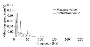 Figure 18 Second-deck crew room
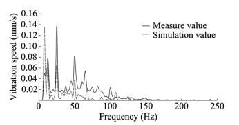 Figure 19 Third-deck stern storage
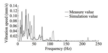 Figure 20 Fourth-deck passenger compartmentTable 1 Comparison of the simulation and test values of the cabin vibration velocity
Location Test value (mm/s) Simulationvalue (mm/s) Tolerance Second-deck laundry room 0.09 0.08 6% Second-deck crew room 0.15 0.13 13% Third-deck stern storage 0.23 0.18 21% Fourth-deck passenger cabin 0.22 0.26 18% 4 Analysis of the contribution of the excitation source to the structural underwater acoustic radiation
In general, the sound pressure level distribution of multiple sources in the far-field region of their synthetic sound field roughly satisfies the linear superposition principle. The total sound level of underwater acoustic radiation noise can be obtained by the linear superposition of a single radiated noise, and the contribution of the acoustic radiation generated by a single excitation source to the total acoustic radiation can be obtained by the equation
$$ \eta = \frac{{{E_n}}}{{\sum\limits_{i = 1}^N {{E_i}} }} = \frac{{p_n^2}}{{p_{{\rm{eng }}}^2 + p_{{\rm{pro }}}^2}} \times 100\% {\rm{(}}n = {\rm{ eng, pro)}} $$ (20) where peng and ppro are the radiated sound pressure caused by the main engine and propeller excitation, respectively, which can be obtained by loading the forces excited by the main engine and propeller separately.
Through the calculation, the sound pressure distribution of X-BOW near the sound field is obtained, and the sound pressure distribution clouds of the typical frequency points of 12.5, 17.5, 67.5, and 110 Hz are selected (Figure 21). In accordance with the characteristics of the sound pressure distribution, three points are selected at the stern, amidship, and bow (Figure 22). The sound pressure at these points is calculated by separately loading the forces excited by the main engine and propeller and brought into Equation (20). The contribution rate of the main engine and propeller excitation to the far field underwater sound radiation can be found (Table 2). At the stern position, the near-field noise is dominated by the sound radiation generated by propeller excitation. At the amidships position, the nearfield noise is dominated by the sound radiation generated by the main engine excitation. At the bow position, the sound radiation generated by propeller excitation is slightly larger than that generated by the main engine excitation. The main reasons for the above phenomenon are as follows: In the X expression in Equation (3), the magnitude of sound pressure at the measurement point is inversely proportional to the distance from the measurement point to the sound source, and the propeller is located at the stern position. Thus, the near-field noise at the stern is dominated by the sound radiation generated by the propeller excitation. Similarly, the main engine is located amidships, and thus, the near-field noise amidships is dominated by the sound radiation generated by the main engine excitation. Therefore, at the bow, the acoustic radiation generated by the propeller excitation is slightly larger than that generated by the main engine excitation (Nikiforov, 1988).
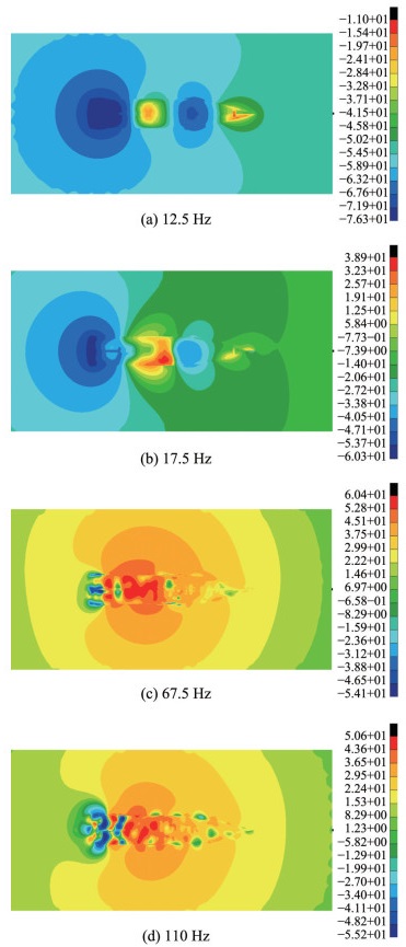 Figure 21 Near-field cloud map distribution
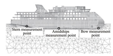 Figure 22 Near-field measurement point arrangementTable 2 Contribution of excitation source to near-field underwater acoustic radiation
Location Acoustic radiation frommain engine excitation (Pa) Contribution of main engine excitation (%) Acoustic radiation from propeller excitation (Pa) Contribution rate of propeller excitation (%) Bow 0.012 45.3 0.013 54.7 Amidships 0.105 90.3 0.034 9.7 Stern 0.045 4.3 0.212 95.7 The sound source far-field directivity of the three surfaces is calculated (Figure 23). The strongest sound radiation is detected at 180° in the horizontal plane, middle longitudinal section, and 190° in the middle transverse section. These three far-field points are used. The host- and propellerexcited forces are loaded separately for the calculation of the sound pressure and brought into Equation (20). Host and propeller excitation on the far-field are achieved. As shown in Table 3, the contribution of propeller excitation to underwater far-field noise is much greater than the contribution of host excitation to underwater far-field noise because the main frequency of the propeller is reduced, and the number of waves generated and the loss during propagation are small.
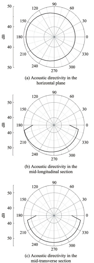 Figure 23 Far-field sound directivityTable 3 Contribution of excitation source to far-field underwater acoustic radiation
Location Acoustic radiation from main engine excitation (Pa) Contribution rate of main engine excitation (%) Acoustic radiation from propeller excitation (Pa) Contribution rate of propeller excitation (%) Horizontal plane 180° 0.002 0 12.7 0.005 2 87.3 Mid-longitudinal section 190° 0.004 0 12.8 0.010 4 87.2 Mid-horizontal section 190° 0.003 6 17.3 0.007 9 82.7 5 Conclusions
An FEM–BEM model of the X-BOW-type polar expedition cruise ship was established and used in the analysis of the main excitation force of a whole ship. Based on the FEM–BEM model and the excitation force, research on the underwater acoustic radiation of the X-BOW-type polar expedition cruise ship was carried out. The specific work and conclusions were as follows:
1) The finite element model of the 100 m X-BOW polar exploration cruise was established. In addition, the underwater sound field of the X-BOW polar exploration cruise was established with the direct boundary method, including the near sound field and far sound field.
2) Vibration velocity at the bottom plate above the propeller and the base of the main engine was tested, and the transfer path admittance from the excitation point to the vibration velocity measurement point was calculated using the finite element model of the X-BOW polar exploration cruise. Moreover, the coherence between each excitation source was analyzed, and propeller pulsation excitation and main engine excitation were inverted through traditional transfer path analysis. The two excitation sources were loaded in the finite element model. The simulated values of the vibration response of four compartments were compared with the tested values. The trend of the frequency response curve was basically the same, and the error of the effective value of the vibration response was within 21%, meeting the required engineering accuracy and verifying the accuracy of propeller pulsation excitation and main engine excitation.
3) Using the obtained excited force, we calculated the X-BOW polar exploration cruise near-field and far-field low-frequency underwater noise. The maximum value of near-field radiation sound pressure was mainly found under the bottom of the ship, and the sound pressure distribution was flap-shaped. The flap-shaped distribution decreased with increasing frequency and tended to be non-uniform. The maximum value of far-field radiation sound pressure was mainly found in the waterline surface (180°), midlongitudinal profile (190°), and mid-transverse profile (190°).
4) Using the linear superposition principle, we loaded the main engine and propeller excitation separately. The contributions of the two excitation sources to the underwater noise were calculated. At the stern position, the nearfield noise was dominated by the sound radiation generated by the propeller excitation, accounting for 95.7%, and at the midship position. The near-field noise was dominated by the sound radiation generated by the main engine excitation, accounting for 90.3%. The sound radiation from propeller excitation accounted for 54.7%, and that from main engine excitation accounted for 45.3%. For far-field underwater noise, the contribution of propeller excitation to underwater noise was much larger than that of host excitation to underwater noise, which accounted for a maximum of 87.3%. According to the above conclusions, the underwater noise of the X-BOW polar exploration cruise can be controlled in a targeted manner.
Competing interest The authors have no competing interests to declare that are relevant to the content of this article. -
Figure 1 Finite baffle placed in the fluid
Figure 2 X-BOW polar exploration cruise underwater acoustic radiation model
Figure 3 X-BOW polar exploration cruise finite element model
Figure 4 Transmission pathway analysis schematic
Figure 5 Vibration velocity of the ship bottom plate directly above the propeller
Figure 6 Propeller pulsation excitation area map
Figure 7 Propeller pulsation excited force area division
Figure 8 Transfer path admittance of each propeller excited force area on the starboard side to measurement point 1
Figure 9 Comparison of transfer path admittance from excitation source to measurement point 1
Figure 10 Propeller pulsation excitation
Figure 11 Schematic diagram of main engine vibration isolator installation
Figure 12 Finite element model of mainframe base and measurement point arrangement
Figure 13 Vibration velocity of measurement point 1 and measurement point 7
Figure 14 Transfer path admittance from measurement points 1, 13, and 19 to measurement point 1
Figure 15 Transfer path admittance from measurement points 1 to 3, 4, 7–9, and 10 to measurement point 1
Figure 16 Main engine–excited force
Figure 17 Second-deck laundry room
Figure 18 Second-deck crew room
Figure 19 Third-deck stern storage
Figure 20 Fourth-deck passenger compartment
Figure 21 Near-field cloud map distribution
Figure 22 Near-field measurement point arrangement
Figure 23 Far-field sound directivity
Table 1 Comparison of the simulation and test values of the cabin vibration velocity
Location Test value (mm/s) Simulationvalue (mm/s) Tolerance Second-deck laundry room 0.09 0.08 6% Second-deck crew room 0.15 0.13 13% Third-deck stern storage 0.23 0.18 21% Fourth-deck passenger cabin 0.22 0.26 18% Table 2 Contribution of excitation source to near-field underwater acoustic radiation
Location Acoustic radiation frommain engine excitation (Pa) Contribution of main engine excitation (%) Acoustic radiation from propeller excitation (Pa) Contribution rate of propeller excitation (%) Bow 0.012 45.3 0.013 54.7 Amidships 0.105 90.3 0.034 9.7 Stern 0.045 4.3 0.212 95.7 Table 3 Contribution of excitation source to far-field underwater acoustic radiation
Location Acoustic radiation from main engine excitation (Pa) Contribution rate of main engine excitation (%) Acoustic radiation from propeller excitation (Pa) Contribution rate of propeller excitation (%) Horizontal plane 180° 0.002 0 12.7 0.005 2 87.3 Mid-longitudinal section 190° 0.004 0 12.8 0.010 4 87.2 Mid-horizontal section 190° 0.003 6 17.3 0.007 9 82.7 -
Cinkraut J (2016) Transfer path analysis of a passenger. PhD thesis, Royal Institute of Technology, Stockholm Det NV (1983) Prevention of harmful vibration in ships. Maritime Technical Information Facility, Oslo Frank F, Paolo G (2006) Sound and structural vibration. Academic Pr, Elsevier Fu ZJ, Xi Q, Li YD, Huang H, Rabczuk T (2020) Hybrid FEM-SBM solver for structural vibration induced underwater acoustic radiation in shallow marine environment. Computer Methods in Applied Mechanics and Engineering 369: 113236. DOI: 10.1016/j.cma.2020.113236 Fu ZJ, Xi Q, Gu Y, Li J, Qu W, Sun L, Wei X, Wang F, Lin J, Li W (2023) Singular boundary method: A review and computer implementation aspects. Engineering Analysis with Boundary Elements 147: 231–266. DOI: 10.1016/j.enganabound.2022.12.004 Gao C, Zhang H, Li H, Pang F, Wang H (2022) Numerical and experimental investigation of vibro-acoustic characteristics of a submerged stiffened cylindrical shell excited by a mechanical force. Ocean Engineering 249: 110913. DOI: 10.1016/j.oceaneng.2022.110913 Hajime T (1976) Estimate of surface force induced by propeller. The Society of Naval Architects of Japan: Tokyo, 140: 49–67. DOI: 10.2534/JJASNAOE1968.1976.140_67 He ZY (1981) The theoretical basis of acoustics. Defense Industry Press, Beijing Jin XD, Xia LJ (2011) Hull vibration. Shanghai Jiao Tong University Press, Shanghai Kehr YZ, Kao JH (2011) Underwater acoustic field and pressure fluctuation on ship hull due to unsteady propeller sheet cavitation. Journal of Marine Science & Technology 16: 241–253. DOI: 10.1007/s00773-011-0131-4 Nikiforov AC (1988) Acoustic design of hull structure. National Defense Industry Press, Beijing Su J, Lei Z, Qu Y, Hua H (2018) Effects of non-axisymmetric structures on vibro-acoustic signatures of a submerged vessel subject to propeller forces. Applied Acoustics 133: 28–37. DOI: 10.1016/j.apacoust.2017.12.006 Wang XZ, Jiang QZ, Xiong YP, Gu X (2020) Experimental studies on the vibro-acoustic behavior of a stiffened submerged conicalcylindrical shell subjected to force and acoustic excitation. Journal of Low Frequency Noise, Vibration and Active Control 39(2): 280–296. DOI: 10.1177/1461348419844648 Wu J, He T, Wang WB (2019) Verification of underwater acoustic radiation calculation method based on Abaqus for water-filled double hull on sideboard. China Shipbuilding 60(1): 175–184. (in Chinese) DOI: CNKI:SUN:ZGZC.0.2019-01-017 Zou MS, Tang HC, Liu SX (2023) Modeling and calculation of acoustic radiation of underwater stiffened cylindrical shells treated with local damping. Marine structures 88: 103366. DOI: 10.1016/j.marstruc.2022.103366
