1   Introduction

Oil spills at sea have the characteristics of long hazard time and large influence degree, causing serious harm to the marine environment and biological health. For example, oil spills cut off the contact between seawater and air, thereby reducing the oxygen content of seawater and endangering the growth of marine organisms. The cyclic aromatic hydrocarbons in oil spills increase the probability of cancer and genetic mutation in mammals. Oil spills can also hinder the heat exchange between the ocean and the atmosphere (Bucas and Saliot, 2002; Liu and Tian, 2006; Lee and Jung, 2015). Therefore, quickly and effectively dealing with an oil spill accident is of great significance. Commonly used oil spill treatment measures mainly include physical, chemical, and biological methods; among them, the physical method is the most ideal and includes the use of booms for containment and recovery and the adsorption of oleophilic materials (Zhang et al., 2020). Collecting and recovering oil spills by manned ships carrying oil booms is one of the commonly used techniques; however, it consumes substantial manpower and material resources and causes serious injuries to the staff on board unmanned surface vehicles (USVs) offer advantages such as miniaturization, autonomy, modularity, strong maneuverability, and high endurance (Manley, 2008; Liao, 2012; Liao et al., 2019). Using USVs instead of manned ships to recover oil spills at sea has many advantages, including avoiding human involvement, lowering recovery costs, improving the efficiency of task execution, and avoiding further volatilization and expansion of oil spills caused by prolonged recovery time. Hence, this approach has great practical application.

Reasonable path planning in oil spill recovery can ensure the safe and efficient completion of the task of USVs, which has great research significance and practical application. It is a system optimization problem with complex constraints (Drake et al., 2018; Yuan et al., 2019). Wang (2015) proposed a USV formation path planning algorithm based on the variable fast marching square method; it changes the anisotropy of the feasible region according to the set way so the final planned path can be balanced between the path length and safety. Considering that USVs are limited by motion constraints, Liu and Richard (2016) proposed an angle-guided fast marching square method to ensure that the generated path conforms to the dynamics and orientation constraints of the USV. For cooperative path planning considering the heterogeneity of USVs, Tan et al. (2020) established a path evaluation function based on the fast marching square method to quantify the matching degree of expected paths with different characteristics relative to the heterogeneous type of USVs. Hence, a global expected path that can unify and coordinate the characteristics of each USV in the cluster can be planned. Sang et al. (2021) proposed a hybrid path planning algorithm based on improved A* and multiple subtarget artificial potential field (APF), which can greatly reduce the probability of USVs falling into the local minimum and help the USVs escape from the local minimum by switching the target point. Aiming at the water–air cooperative operation task of unmanned aerial vehicles and USVs, Zheng et al. (2021) adopted a combination of virtual structure and APF control algorithm. The formation of vehicles is organized through the virtual structure method, and the state error of vehicles and APF function are utilized to achieve preset formation and avoid collision between unmanned aerial vehicles.

In summary, research on the cooperative path planning of multiple USVs is mainly based on the improved APF method, the improved A* algorithm, and the fast marching flat method. Traditional A* method (Hao and Agrawal, 2005), particle swarm optimization algorithm (Duan et al., 2008), genetic algorithm (Qu et al., 2013), and ant colony algorithm (Asl et al., 2013) are also used to study the cooperative path planning problem of multirobots but are rarely applied to the research on the collaborative path planning of USVs.

Compared with other path planning algorithms, the more widely used APF method has the advantages of simpler principles, faster calculation speed, and better real-time performance. Orozco-Rosas et al. (2019) combined membrane computing with a genetic algorithm and the APF method to propose a membrane evolutionary APF approach for solving the problem of mobile robot path planning. This method has shown improved performance in terms of path length and timeliness. By combining the APF method and the Deep Deterministic Policy Gradient (DDPG) algorithm, Li et al. (2023) proposed an improved algorithm APF-DDPG to improve the obstacle avoidance trajectory planning capability of mobile robotic arms in narrow passage and obstacle constraints. Compared with traditional DDPG, the improved algorithm can be trained with higher convergence efficiency to obtain a policy model with more efficient control performance. Orozco-Rosas et al. (2022) utilized the APF method to improve the classical Q-learning approach for solving the limitation of slow convergence to the optimal solution. Experiments demonstrate that in offline and online path planning modes, the Q-learning algorithm combined with the APF method algorithm successfully achieves better learning values and outperforms the classical Q-learning approach in all test environments.

The APF method also has problems, such as local minimum and unreachable targets, both of which have been studied by scholars. Jiang (2020) improved the potential function of the repulsive field to solve the local minimum problem of the APF method and applied it to the path planning of oil spill recovery systems. Experimental results show that the system can successfully avoid obstacles and finally return to the original trajectory. Sun et al. (2022) introduced the Bug algorithm to ensure the global performance of the proposed algorithm in addressing the problem of the traditional APF method easily falling into the local minimum. Test results show that the improved algorithm effectively enhances the safety of the intelligent vehicle during driving and allows the vehicle to overtake smoothly. Chu (2022) designed the expected heading compensation method to solve the large inflection point problem by smoothening the path while improving the repulsive field; however, the performance constraints of the double USV system were not considered. Current improvement methods for the traditional APF method mostly aim to improve a certain flaw of APF; this approach is not comprehensive enough and still allows room for improvement.

Herein, the path planning of the double USV oil spill recovery system (DUOSRS) is studied with the engineering background of oil spill recovery by double USVs towing oil booms. Figure 1 shows the whole process of the oil spill recovery of the DUOSRS, including approaching the target oil spill, rounding up the target oil spill, and consigning the target oil spill to the recovery site (Giron-Sierra et al., 2014). Considering the influence of obstacles on oil spill recovery, this research uses the improved APF method for path planning. After the three flaws of this method are analyzed, three improved algorithms are proposed by combining the motion performance constraints of the DUOSRS. The APF-123 algorithm for oil spill recovery is then established by combining these three algorithms. In consideration of the flaws of the APF and the process of oil spill recovery, multiple sets of simulation tests are designed. Results show that the proposed algorithms can ensure the safety of the system to track the oil spill in environments with numerous obstacles and increase the speed and success rate of the task.

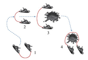Figure  1  Diagram of double USV system for oil spill recovery

Download: Full-Size Img

2   Principles and flaws of APF

Owing to the wide area covered by the DUOSRS during sailing, the influence of obstacles in the path must be considered. Compared with other classical path planning algorithms, the APF method has the advantages of simpler principles, faster calculation speed, and better real-time performance. Hence, this work uses this method for the path planning of the double USV system.

First proposed by Khatib in 1986, the APF is a virtual force method (Khatib, 1986; Yu and Lu, 2021; Liu and Dou, 2021) for simulating natural fields. In this method, obstacles, target points, and USVs are treated as points, and the USV moves in a virtual force field composed of attractive and repulsive potential fields. The attractive potential field around the target point has an attractive effect on the USV, and the repulsive potential field around the obstacle has a repulsive effect on the USV. Figure 2 shows that under the combined force of attraction and repulsion, the USV avoids obstacles and tends to approach the target. The principle of the APF method is as follows:

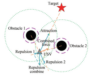Figure  2  Force diagram of the USV

Download: Full-Size Img

where U is the combined potential field, U_att is the attractive potential field, and U_rep is the repulsive potential field. The directions of the negative gradient of the above three potential fields are the directions of the combined force, attractive force, and repulsive force.

1) Attraction calculation

The APF function of the target point to the USV is as follows:

where k_att is the attraction gain constant, X_t is the position of the target point, and X is the position of the USV.

The attraction direction of the target point on the USV is the direction of the negative gradient of the attractive potential field. The calculation formula for the attraction is as follows:

2) Repulsion calculation

The repulsive potential field function of the obstacle to the USV is as follows:

where k_rep is the repulsion gain constant, ρ_obs is the distance between the USV and the obstacle, and ρ₀ is the influence radius of the obstacle.When the distance between the USV and the obstacle is greater than ρ₀, the USV is not subject to the repulsive force of the obstacle.

The repulsion direction of the obstacle to the USV is the negative gradient direction of the repulsive potential field. The calculation formula for the repulsion force is as follows:

The combined force of repulsion and attraction on the USV at its position X is as follows:

The APF method has been widely used because of its advantages of simple calculation and easy implementation. However, this method also has certain flaws (Figure 3), which are summarized as follows:

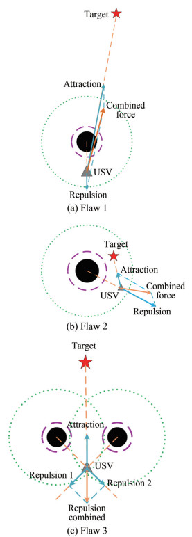Figure  3  Diagram of the three flaws of the APF method

Download: Full-Size Img

1) Flaw 1: when the distance between the USV and the target is greater than the distance between the USV and the obstacle, the attractive force of the target point on the USV is greater than the repulsive force of the obstacle on the USV and the USV is very likely to collide with the obstacle;

2) Flaw 2: when the target point is within the influence distance of the obstacle and close to the obstacle, the repulsive force of the obstacle on the USV is greater than the attractive force of the target point on the USV and the USV cannot reach the target point;

3) Flaw 3: in tracking the target, the combined force of the repulsion and attraction on the USV might be zero in one position, and the USV will stop moving because it falls into the local minimum point.

Among these flaws 1 and 2 can be summarized as unreachable target problems, and 3 can be summarized as a local minima problem.

3   Improved APF algorithm for oil spill recovery

In this section, an improved algorithm APF-123 is proposed for the path planning of the system by combining the motion performance constraints of the DUOSRS with the three flaws of the APF method described in the previous section.

3.1   Definition of the virtual pilot

When the formation center of the double USVs in the oil spill recovery system is set as the virtual pilot (Jiang, 2020), the path planning of the DUOSRS can be simplified to that of the virtual pilot. As shown in Figure 4, USV1's coordinates are (x₁, y₁), its heading is ψ₁, and its speed is v₁. USV2's coordinates are (x₂, y₂), its heading is ψ₂, and its speed is v₂. The virtual pilot's coordinates are (x_v, y_v), the heading is ψ_v, and the speed is v_v. The three relationships are as follows:

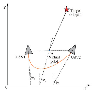Figure  4  Diagram of the virtual pilot

Download: Full-Size Img

3.2   Obstacle model of the DUOSRS

The virtual pilot is taken as the research object to simplify the calculation. However, in an actual situation, the DUOSRS covers a wide area of the sea and cannot be simplified into a single point for calculation; otherwise, a situation will arise where the virtual pilot can avoid the obstacles, but the DUOSRS will collide with the obstacles. To solve the above problems, the safety compensation radius for the formation of double USVs is added to the obstacle model of the traditional APF method. As shown in Figure 5, the actual radius of the obstacle is r_obs, the influence radius of the obstacle is ρ₀, and the safety compensation radius is r_s. In the subsequent research, the equivalent radius r_o = r_obs + r_s of the obstacle will be calculated instead of the actual radius to avoid the above situation.

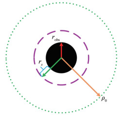Figure  5  Diagram of the obstacle model

Download: Full-Size Img

3.3   Improved algorithm APF-123

Combined with the obstacle model, three algorithms, APF-1, APF-2, and APF-3, are proposed by improving the three flaws of the traditional APF method, respectively. Finally, the APF-123 algorithm is put forward by combining these three algorithms.

3.3.1   Improved algorithm for flaw 1

The improved algorithm for flaw 1 of the traditional APF method (APF-1) is shown in Figure 6, where the position of the virtual pilot is V (x_v, y_v), that of the obstacle is R(x_obs, y_obs), and that of the target point is T (x_t, y_t); ρ_obs is the distance between the virtual pilot and the obstacle; ρ_ot is the distance between the target point and the obstacle; ρ₀ is the influence radius of the obstacle; r_obs is the actual radius of the obstacle; r_o is the equivalent radius of the obstacle; F is the combined force of attraction F_att and repulsion F_rep; l is the vertical distance of the obstacle to the line where F is located; Γ is the introduced safety compensation distance for flaw 1; S is the point obtained by extending the equivalent radius r_o of the obstacle Γ along the direction l; β is the angle between the line VR and the X-axis; μ is the angle between the line VR and the direction F; θ is the angle between F and the X-axis; γ is the angle corresponding to the side RS in ΔVRS; and ε is the angle corresponding to the side VS in ΔVRS.

After calculation, the relationship between the above parameters can be obtained as follows:

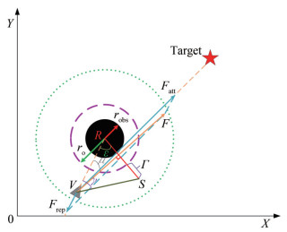Figure  6  Diagram of the APF-1 algorithm

Download: Full-Size Img

The improved part of the APF-1 algorithm is shown in the following Table 1:

where φ_ox is the angle between the pilot's heading and the X-axis in Figure 6.

The introduced safety compensation distance Γ of the APF-1 algorithm is used to limit the minimum vertical distance between the obstacle and the line where F is located. According to Table 1, when ρ_ot > ρ₀, μ < $\frac{\pi}{2}$ and l < r_obs + r_s + Γ, φ_ox = β − γ, the virtual pilot sails away from the obstacle, effectively avoiding flaw 1.

According to Figure 6, the above discussion pertains to the case where the center point (x_obs, y_obs) of the obstacle is above the line between the virtual pilot and the target point. The analysis process for the other case is similar and will not be repeated.

3.3.2   Improved algorithm for flaw 2

The improved algorithm for flaw 2 of the traditional APF method (APF-2) is shown in Figure 7, where the position of the virtual pilot is V (x_v, y_v), that of the obstacle is R(x_obs, y_obs), and that of the target point is T (x_t, y_t); ρ_vt is the distance between the virtual pilot and the target point; ρ_obs is the distance between the virtual pilot and the obstacle; ρ_ot is the distance between the target point and the obstacle; ρ₀ is the influence radius of the obstacle; r_obs is the actual radius of the obstacle; r_o is the equivalent radius of the obstacle; d is the vertical distance from the obstacle to the connection between the virtual pilot and the target point; Ω is the introduced safety compensation distance for flaw 2;Q is the point obtained by extending the equivalent radius r_o of the obstacle Ω along the direction d; β is the angle between the line VR and the X-axis; η is the angle between the line VT and the X-axis; σ is the angle corresponding to the side VQ in ΔVRQ; γ₁ is the angle corresponding to the side RQ in ΔVRQ; and λ is the angle corresponding to the side RT in ΔVRT.

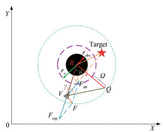Figure  7  Diagram of the APF-2 algorithm

Download: Full-Size Img

After calculation, the relationship between the above parameters can be obtained as follows:

When ρ_ot < ρ₀, the virtual navigator falls into flaw 2. The improved part of the APF-2 algorithm is shown in the following Table 2:

where φ_ox is the angle between the pilot's heading and the X-axis in Figure 7.

The introduced safety compensation distance Ω of the APF-2 algorithm is used to limit the minimum vertical distance from the obstacle to the connection between the virtual pilot and the target point. Table 2 shows that when d ≥ r_obs + r_s + Ω or λ ≥ $\frac{\pi}{2}$, φ_ox = η, the virtual pilot approaches the target point directly along the line direction with the target point. Otherwise, φ_ox = β − γ₁, in which the virtual pilot approaches the target point while avoiding obstacles, effectively avoiding flaw 2.

According to Figure 7, the above discussion pertains to the case where the center point (x_obs, y_obs) of the obstacle is above the line between the virtual pilot and the target point. The analysis process for the other case is similar and will not be repeated.

3.3.3   Improved algorithm for flaw 3

Flaw 3 describes the situation where the virtual pilot may stop moving due to the local minimum point while tracking the target. The improved algorithm for flaw 3 of the traditional APF method (APF-3) is combined with the simulated annealing (SA) algorithm to improve the APF method and then with the motion performance constraints of the DUOSRS to screen the next position of the virtual pilot selected by the SA algorithm. This approach ensures that the path near the local minimum point will not exhibit large oscillation, and the DUOSRS can accurately track the planned path.

1) Principle of the SA algorithm

The Metropolis criterion is the basis of the SA algorithm, that is, to accept a new state with a certain probability. Assume the current state of the research object is Φ (k) and the state of the research object at the next moment is Φ (k + 1); according to the energy of gradient descent, the energy of the research object also changes from E (n) to E (n + 1). According to the Metropolis criterion, the change in the acceptance probability of the state of the research object changing from Φ (k) to Φ(k + 1) is defined as follows:

where T is the temperature in the SA algorithm reduced in a certain way, as shown in the following formula:

where α is an arbitrary positive constant of the interval (0.85, 1) selected according to the actual situation, and t is the number of iterations.

Formula (11) indicates that if the energy goes down, then the acceptance probability of the state of the research object from Φ(k) to Φ(k+1) is 1; that is, it can be accepted. If the energy increases, it will be accepted with a certain probability. A random probability ξ is set. When P >ξ, accept the state of the research object from Φ (k) to Φ (k + 1); otherwise, proceed to the next step (Zang et al., 2021; Liu et al., 2021; Han, 2021).

2) APF-3 algorithm

When the local minimum point is removed by the APF method based on SA, the virtual pilot will have a relatively violent oscillation near the local minimum point, which easily causes "entanglement" and "towing separation" in the tracking of the DUOSRS and then the failure of the recovery task. Combined with the maximum heading change angle of the DUOSRS, the next position of the virtual pilot selected by the SA algorithm is screened twice to ensure that the path planning near the local minimum point is in line with the motion performance constraints of the double USV system and no large oscillation appears so that the DUOSRS can accurately track the planned path. The maximum heading change angle of the DUOSRS is calculated as follows:

Here, φ_m is the maximum heading change angle of the DUOSRS, R_s is the turning radius of the USV located outside the DUOSRS at the current moment, Δt is the time step, and v_v is the speed of the virtual pilot.

The secondary screening mechanism is shown in Table 3.

In the table, φ_Δ is the absolute value of the change in the heading angle of the DUOSRS.

The specific steps for the APF-3 algorithm to escape from the local minimum point are as follows:

Step 1: Perform parameter initialization to determine the initial temperature T₀, termination temperature T_f, random probability ξ, and maximum heading change angle φ_m of the DUOSRS.

Step 2: Select a random point X₁ near the virtual pilot's current position V.

Step 3: Calculate the potential field of the position V and position X₁ as U (V) and U (X₁) respectively. If U (X₁) − U (V) < 0, then the next position of the virtual pilot is X₁. If U (X₁)− U (V) ≥ 0, then the probability P of accepting X₁ is calculated according to the Metropolis criterion. If P > ξ, then the next position of the virtual pilot is X₁; otherwise, return to step 2 to select a random point again.

Step 4: Before accepting X₁ as the next position of the virtual pilot, calculate the difference φ_Δ between the current and next position heading of the virtual pilot and compare it with φ_m. If φ_Δ ≤ φ_m, then accept the next position of the virtual pilot as X₁; otherwise, return to step 2 to select a random point again.

Step 5: After the virtual pilot reaches the position X₁, determine whether the combined force of attraction and repulsion on the virtual pilot's position is 0. If the combined force is not 0, then the virtual pilot eliminates the local minimum point and keeps tracking the target point; otherwise, return to step 2 to select a random point again.

The flow chart of the APF-3 algorithm out of the local minimum point is shown in Figure 8.

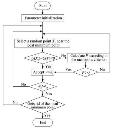Figure  8  Flow chart of the APF-3 algorithm

Download: Full-Size Img

The APF-123 algorithm for oil spill recovery is obtained by combining the above three algorithms, and its flow chart is shown in Figure 9.

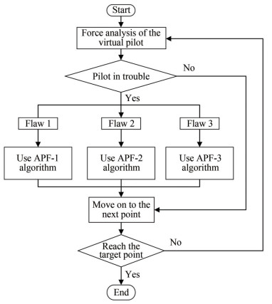Figure  9  Flow chart of the APF-123 algorithm

Download: Full-Size Img

4   Simulation tests and results

Simulation tests are designed and carried out in the following four parts to verify the effectiveness and feasibility of the improved algorithms:

1) The APF-1 algorithm and APF method are compared under the condition of flaw 1 to verify the effectiveness of the APF-1 algorithm;

2) The APF-2 algorithm and APF method are compared under the condition of flaw 2 to verify the effectiveness of the APF-2 algorithm;

3) The APF-3 algorithm, APF method, and APF algorithm based on SA are compared under the condition of defect 3 to verify the effectiveness of the APF-3 algorithm;

4) The APF-123 algorithm is used for the tracking and obstacle avoidance tests of dynamic targets to verify its feasibility and effectiveness when applied to the oil spill recovery system.

4.1   Simulation comparison test under the condition of flaw 1

The starting position of the virtual pilot is (0, 0), the position of the target point is (350, 350), the position of the obstacle is (50, 50), the actual radius of the obstacle r_obs = 15 m, the safety compensation radius r_s = 5 m, the influence radius of the obstacle ρ₀ = 30 m, the attraction gain constant k_att = 10, the repulsion gain constant k_rep = 5 × 10⁵, and the safety compensation distance Γ = 6 m in the APF-1 algorithm. The simulation result is shown in Figure 10.

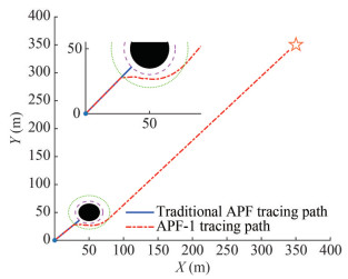Figure  10  APF and APF-1 tracking paths under the condition of flaw 1

Download: Full-Size Img

Figure 10 shows that under the condition of flaw 1, the tracking path planned by the APF method crashes into the equivalent radius of the obstacle, resulting in the failure of the tracking task of the virtual pilot. By contrast, the tracking path planned by the APF-1 algorithm always maintains a safe distance of no less than 6 m from the equivalent radius of the obstacle. In addition, the virtual pilot is still able to track the target point under the condition of flaw 1, ensuring the successful completion of the oil spill recovery task.

4.2   Simulation comparison test under the condition of flaw 2

The starting position of the virtual pilot is (0, 0), the position of the target point is (200, 200), the position of the obstacle is (175, 200), the actual radius of the obstacle r_obs = 10 m, the safety compensation radius r_s = 5 m, the influence radius of the obstacle ρ₀ = 45 m, the attraction gain constant k_att = 10, the repulsion gain constant k_rep = 4 × 10⁶, and the safety compensation distance Ω = 8 m in the APF-2 algorithm. The simulation result is shown in Figure 11(a).

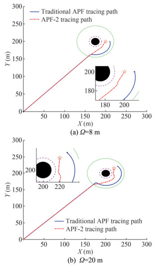Figure  11  APF and APF-2 tracking paths under the condition of flaw 2

Download: Full-Size Img

In the above simulation conditions, the position of the target point is changed to (220, 215), that of the obstacle is changed to (200, 200), and the safety compensation distance is Ω = 20 m in the APF-2 algorithm. The simulation comparison test is conducted, and the result is shown in Figure 11(b).

Figure 11 shows that when the target point is located within the influence distance of the obstacle and relatively close to the equivalent radius of the obstacle, the path planned by the APF method causes the "unreachable target" phenomenon. When the repulsive force received by the virtual pilot is greater than the attractive force, the virtual pilot oscillates irregularly in a small area when it is still a distance away from the target point, leading to the failure of the tracking task. The APF-2 algorithm allows the virtual pilot to track the target point while maintaining a certain safe distance from the equivalent radius of the obstacle, ensuring the success of the oil spill recovery task. In addition, the planned paths are shortened, which reduces energy consumption. Compared with the APF method, the APF-2 algorithm has better practicality.

4.3   Simulation comparison test under the condition of flaw 3

The starting position of the virtual pilot is (0, 0); the position of the target point is (240, 240); the positions of the obstacles are (40, 40), (120, 60), (60, 120), (100, 100), and (180, 180); the actual radius of the obstacle r_obs = 5 m; the safety compensation radius r_s = 5 m; the influence radius of the obstacle ρ₀ = 25 m; the attraction gain constant k_att = 10; the repulsion gain constant k_rep = 5 × 10⁵, the initial temperature of the APF-3 algorithm and APF algorithm based on SA is 10; the termination temperature is 0.1; and the random probability is ξ = 0.9. The simulation result is shown in Figure 12.

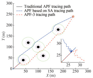Figure  12  Tracking paths of APF, APF based on SA, and APF-3 under the condition of flaw 3

Download: Full-Size Img

Figure 12 shows that the path planned by the APF method causes the virtual pilot to fall into the local minimum point and stop moving, resulting in task failure. Meanwhile, the path planned by the APF algorithm based on SA oscillates violently near the local minimum point, leading to "entanglement" and "towing separation" in the tracking of the DUOSRS and, consequently, the failure of the recovery task. The path planned by the APF-3 algorithm is relatively stable and has less oscillation near the local minimum point, meeting the motion performance constraints of the system and ensuring the success of the task. The effectiveness of the APF-3 algorithm in the oil spill recovery task of double USVs is verified by comparing the result with the tracking paths planned by the APF method and APF algorithm based on SA.

4.4   Dynamic target tracking and obstacle avoidance test

Oil spills in the ocean drift and expand due to the influence of the environment. Given that the virtual pilot is tracking the centroid of the oil spill coverage area and the expansion and drift of the oil spill causes the movement of the centroid, studying the static target tracking is not enough. The following is the dynamic target tracking simulation test.

4.4.1   Target tracking test in a static obstacle environment

The starting position of the virtual pilot is (0, 0), and that of the dynamic target point is (220, 220); the positions of the obstacles are (30, 40), (60, 80), (120, 40), (190, 180), (150, 125), (115, 90), (75, 150), (120, 160), (210, 110), (175, 50), and (150, 200); the actual radius of the obstacle r_obs = 5 m; the safety compensation radius r_s = 5 m; the influence radius of the obstacle ρ₀ = 25 m; the attraction gain constant k_att = 10; the repulsion gain constant k_rep = 5 × 10⁵; the initial temperature of APF-123 algorithm is 10; the termination temperature is 0.1; and the random probability ξ=0.9.

1) Simulation test of regular motion of the target

The speed of the target is set as v_t = 0.2 m/s, the heading of the target is set as φ_t = 120°, i.e. moving at an angle of 120° to the X-axis, and the speed of the virtual pilot v_v = 1.0m/s. The result is shown in Figure 13(a).

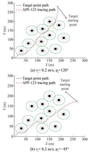Figure  13  APF-123 tracks regularly moving targets in an environment with static obstacles

Download: Full-Size Img

With the other conditions unchanged, the heading of the target is set as φ_t= −45°. The result is shown in Figure 13(b).

Figure 13 shows that the path planned by the APF-123 algorithm allows the virtual pilot to successfully track the regular motion dynamic target under the influence of multiple static obstacles, ensuring the success of the recovery task.

2) Simulation test of the irregular motion of the target Owing to the expansion and drift of the oil spill, the centroid of the oil spill on the sea surface changes irregularly. Hence, a simulation test of the irregular motion of the target point must be carried out. The basic parameters in the simulation are consistent with those for the regularly moving target point described above, with only the speed and direction of the target point being changed. The target is set to move irregularly with a speed v_t = 0.5 × rand (1) m/s along an angle of 270° × rand (1) with the X-axis. The result is shown in Figure 14(a).

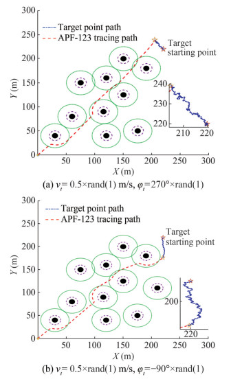Figure  14  APF-123 tracks irregularly moving targets in an environment with static obstacles

Download: Full-Size Img

With the other conditions unchanged, the target is set to move irregularly along an angle of − 90° × rand (1) with the X-axis. The result is shown in Figure 14(b).

Figure 14 shows that the path planned by the APF-123 algorithm allows the virtual pilot to successfully track the irregularly moving dynamic target under the influence of multiple static obstacles, ensuring the success of the recovery task.

4.4.2   Target tracking test in a dynamic obstacle environment

Owing to the presence of other moving objects in the environment and the fact that some marine debris can drift on the surface of the sea under the action of wind and waves, simulation tests in the dynamic obstacle environment must be carried out.

The positions of the three static obstacles are set as (70, 130), (200, 220), and (250, 200), and the initial position of the five dynamic obstacles as (40, 20), (60, 80), (120, 40), (210, 170), and (150, 125). They make uniform linear motion along the angles of 120°, 0°, 60°, −135°, and 90° to the X-axis, respectively, and the speed is 0.2m/s. The starting point of the dynamic target is (220, 220), and it moves irregularly along an angle of − 120° × rand (1) with the X-axis at the speed of v_t = 0.4 × rand(1) m/s. The virtual pilot speed is v_v = 1 m/s. The rest of the parameters are the same as those in 4.4.1. The paths planned using the APF method and APF-123 algorithm are shown in Figures 15(a) and 15(b), respectively.

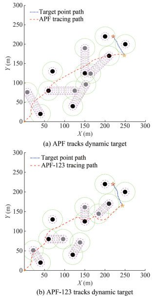Figure  15  APF and APF-123 track dynamic targets in an environment with regular motion obstacles

Download: Full-Size Img

The black circle in the figure indicates the starting position of the obstacle, and the gray circle indicates the position of the obstacle when the virtual pilot tracks the target. In this test, the number of iterative steps to track the target is set to 325 for the APF method and 181 for the APF-123 algorithm, and the efficiency increases by 44.3%.

The dynamic target is set to move irregularly along an angle of 60° × rand (1) with the X-axis, and the dynamic obstacles are set to move along the angles of 180° × rand (1), 0°, 60°, 45° × rand (1), 90° to the X-axis. The rest of the conditions remain unchanged. The paths planned using the APF method and APF-123 algorithm are shown in Figures 16(a) and 16(b), respectively.

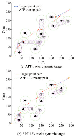Figure  16  APF and APF-123 track dynamic targets in an environment with irregular motion obstacles

Download: Full-Size Img

In this test, the number of iterative steps to track the target is set to 404 for the APF method and 217 for the APF-123 algorithm, and the efficiency increases by 46.3%.

Figures 15 and 16 show that although the path planned by the APF-123 algorithm is not as smooth as that planned by the APF method, the number of iterative steps produced by the APF-123 algorithm is less than 60% that produced by the APF method. In the oil spill recovery task, quickly completing the tracking and reducing the spread of the oil spill are necessary to avoid great pollution, so the APF-123 algorithm with faster speed has better practicality than the APF method.

In summary, comparison tests are set up in sections 4.1– 4.3 for each of the three flaws of the APF method. The results prove that the three improved algorithms can effectively prevent the USVs from falling into the flaws of the APF method and failing the task and improve the success rate of the task, implying their feasibility and practicability. In section 4.4, the dynamic target tracking and obstacle avoidance tests are carried out. The results show that the virtual pilot can track the dynamic oil spill in a complex environment, and the speed is increased by more than 40% compared with that using the APF method. This finding verifies the feasibility and superiority of the APF-123 algorithm for the oil spill recovery system.

5   Conclusions

Against the engineering background of oil spill recovery by double USVs towing oil booms, the path planning of the double USV system for oil spill recovery is studied using the improved APF method. First, the three flaws of the APF method are analyzed in principle, and three improved algorithms are proposed by combining them with the motion performance constraints of the DUOSRS. Second, the APF-123 algorithm for the oil spill recovery system is proposed by combining the three algorithms. Finally, in consideration of the flaws of the APF method and the process of oil spill recovery, several sets of simulation tests under different scenarios are conducted. The results show that the proposed algorithm allows the virtual pilot to safely track the dynamic motion target in a short time, making it a feasible and superior approach.

Although the simulations have successfully accomplished the tracking task, the following are suggested as areas for continued development:

1) Oil spills drift and expand irregularly on the sea surface, and their shape changes irregularly. Hence, tracking the centroid of the oil spill without considering the boundary condition is insufficient. The drift and expansion models of the real oil spill must be considered in subsequent research to achieve high tracking accuracy.

2) In the simulation tests, the position, moving speed, and direction of the obstacle are assumed to be known. In a real marine environment, these parameters may not be accurately measured. Therefore, real ship experiments are warranted to further verify the effectiveness of the proposed algorithm.