1   Introduction

World trade volume has been increasing steadily in recent years. According to the report of the United Nations Conference on Trade and Development (UNCTAD) in 2022, over 80% of global trade is performed by maritime transportation. As an important component of transportation (Umit, 2023), maritime shipping is expected to see an uptick in the number of vessels. The expansion of the fleet leads to heightened traffic density in shipping lanes, which in turn affects the efficiency of vessels traveling in heavily trafficked trade areas. Additionally, rising fuel prices and air pollution pose significant challenges to the shipping industry (Li et al., 2022). The development of the shipping industry has increased energy consumption, generated greenhouse gas emissions, and contributed to the ongoing deterioration of environmental conditions and climate change. Urgent emission reductions within this decade are necessary to mitigate the shipping industry's impact on climate change (James et al., 2023). Therefore, energy-saving and emissionreducing measures for ships and the attainment of sustainable, green development have become essential requirements for the continued growth of the industry. As the world's largest carbon emitter, China has implemented comprehensive measures to reduce greenhouse gas emissions from ships starting from 2023. Considering the important role of the shipping industry in China's economic development and the significance of low-carbon shipping in the country's "dual-carbon" strategy, further research must be conducted on ship shipping efficiency and energysaving and emission-reducing measures.

The route induction problem revolves around ships as the research object. Sailing time, sailing distance, or sailing cost is taken as the induction target to plan the optimal traveling route for the driver to satisfy the conditions. In many cases, the route induction problem can be abstractly considered as the shortest path problem in graph theory. Generally, the optimal driving route can be obtained by combining the ship flow information in the AIS data system with the shortest path algorithm. The main purpose of studying this problem is to provide dynamic navigation services for drivers so that ships can pass through the areas safely, orderly, and timely, thereby improving the efficiency of ship passage and reducing driving accidents (Li et al., 2019). However, the current research on ship route guidance focuses more on navigation efficiency and ignores the environmental impact of carbon emissions during ship navigation. Therefore, the introduction of green navigation in ship route guidance is a direction for future research.

Scholars have proposed theoretical methods for the ship route planning induction problem. Currently, domestic and international research on route guidance for ships mainly focuses on selecting ship routes considering different environmental influences and factors. Tsou et al. (2010) aim to find the shortest navigation path by representing the routes of multiple ships as a series of continuous turning points and using a genetic algorithm to obtain collaborative strategies, thereby calculating the optimal route for ships. Neumann (2015) builds upon Dempster and Shafer evidence theory to induce and optimize ship routes with the objective of shortest paths for ship navigation. Cao (2010) uses an improved particle swarm optimization algorithm to solve the route guidance problem with the objective of minimizing travel time and proposes a method to solve complex nonlinear problems. Du et al. (2018) consider the influence of non-uniform wind fields on route planning and establish an open water sailboat route guidance model with the goal of minimizing travel time, which is solved using an improved genetic algorithm. Zhao (2017) proposes a meteorological route planning algorithm based on the simulated annealing algorithm. They take into account meteorological data obtained from authoritative weather websites and the impact of marine environments on ship movement and conduct simulation analyses for the "most fuel-efficient route model" and "shortest travel time route model". From the perspective of navigation safety, Huang et al. (2018) propose an improved algorithm-based route planning method using weights. They utilize this algorithm to find safe navigation paths, thereby enhancing the efficiency of ship cruising monitoring and ensuring the safety of monitoring tasks during navigation. Liu et al. (2019) consider the route planning problem in continuous construction areas and establish a nonlinear multi-objective ship route planning mathematical model and a route evaluation model with the objectives of minimizing the total route length and path risk value. Finally, they obtain the optimal route through continuous construction areas.

In addition, accurate prediction of ship traffic flow is a prerequisite and key factor for ship traffic guidance. Traffic flow prediction can be divided into long-term and short-term prediction. Long-term prediction covers a longer time span, such as hours, days, months, or even years, and is mainly used for macro-level prediction. Short-term prediction focuses on shorter time spans, usually no more than 15 minutes, and is used for micro-level prediction. For marine traffic flow prediction, the time span for short-term prediction can be extended to one hour because of the wider survey area and relatively fewer ships. Current traffic flow prediction methods can be mainly divided into four categories: linear, nonlinear, intelligent theory-based prediction, and traffic simulation prediction methods. Prediction models based on linear statistical methods mainly include time series, Kalman filtering, and gray models. Differential self-regression moving average models, as a typical time series prediction method, can effectively eliminate the non-smoothness of data (Ma et al., 2020), but the accuracy of such linear prediction methods is low. Nonlinear methods based on neural networks have been gradually becoming a focus of research for scholars owing to their good performance in handling the nonlinearity and complexity of time series data. Considering such good performance, they have a high prediction accuracy for traffic flow. Neural networks, particularly backpropagation (BP) neural networks, are widely applied (Liu et al., 2017). Prediction models based on intelligent theory mainly include deep learning technology and data mining. In the field of deep learning, recurrent neural networks and convolutional neural networks have also achieved good prediction results in ship traffic flow (Dong, 2020). In ship traffic flow prediction research, prediction models based on traffic simulation are utilized. These models focus on the simulation and analysis of ship traffic flow calculations on waterways. Among the numerical simulation methods, the most commonly used research method involves the use of meta-cellular automata. This approach is employed in the simulation and calculation of various aspects, including the maximum throughput capacity of the waterway (Liu et al., 2021) and the evolution of congestion in restricted waterways (Yang et al., 2013).

Research on the sustainable development of maritime logistics has new advancements. De et al. (2021) propose a heuristic program based on the variable neighborhood search algorithm. It addresses environmental issues related to fuel consumption and carbon emissions in the shipping industry while maximizing the operational capabilities of shipping companies. They also develop a mixed-integer nonlinear programming model that considers fuel consumption and speed optimization (De et al., 2020). Non-dominated sorting genetic algorithm and multi-objective particle swarm algorithm are used to address sustainability and safety challenges associated with complex, practical, and realtime maritime transportation problems (De et al., 2019).

In recent years, ship routing has attracted significant attention from scholars domestically and internationally. Despite notable research progress, research on ship route induction remains scarce. Existing studies mostly focus on considering a single factor as the induction objective. Only a small portion of the literature related to maritime logistics considers environmental sustainability issues associated with reducing fuel consumption and carbon emissions. To improve the efficiency of maritime shipping and promote the development of low-carbon shipping, striking a balance between navigation efficiency, energy conservation, and emission reduction is imperative. Therefore, this study proposes a multi-objective ship route dynamic induction method that considers navigation time, distance, and fuel consumption as induction objectives. Providing proper ship route guidance can reduce the sailing time of vessels, improve navigational efficiency, and reduce energy consumption, thereby lowering greenhouse gas emissions and achieving efficient and environmentally friendly shipping. Additionally, to better meet the requirements of ship route guidance, this study utilizes dynamic traffic flow data to calculate the values of the road impedance function within each segment instead of relying on static historical data. This approach marks a significant difference between dynamic induction and static guidance.

2   Multi-section ship short-term traffic flow forecast

On the basis of the summary of various short-term traffic flow prediction methods, this study proposes an improved four-layer hidden node synthetic BP neural network prediction model to address the low prediction accuracy in ship traffic flow prediction. An improved algorithm is introduced in the prediction process to enhance network performance and ultimately improve the accuracy of the prediction model. The improved BP network demonstrates excellent performance in nonlinear fitting, with unique non-convexity, adaptability, robustness, and high fault tolerance. Compared with the commonly used wavelet neural network, the improved four-layer hidden node synthetic BP neural network introduces a momentum term, overcoming the drawbacks of slow evolution and susceptibility to local minima. It also improves the learning efficiency of the network.

2.1   Theoretical basis of the prediction model

The BP neural network is a multi-layer feedforward neural network that originates from the backpropagation algorithm, which is used to adjust the network's weights during training. According to statistics, around 80% of neural network models use the BP network or its variations. The BP network has several advantages, such as good fault tolerance, limited contribution of outliers in the training data, strong immunity to outliers during learning, and robustness. It is currently considered one of the most mature and perfect artificial neural networks. The topology structure of the traditional three-layer BP network is shown in Figure 1.

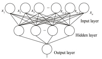Figure  1  Schematic of BP neural network

Download: Full-Size Img

The process of BP neural networks involves continuously adjusting the weights and thresholds by propagating the error backward, aiming to minimize error or approach the desired error level. The reduction of error is typically achieved using the negative gradient descent method. In essence, BP neural networks are highly accurate numerical approximators. The principle behind them is to connect activation functions and adjust the coefficients of these functions to minimize the error as much as possible. The formula for adjusting weights and thresholds in a conventional three-layer BP network is as follows:

where E is the sum of squared errors between the network output and the actual output sample; n is the learning rate of the network, that is, the amplitude of weight adjustment; w_ij (t) is the connection weight between the ith neuron of the layer and the jth neuron of the hidden layer at time t; w_ij (t + 1) is the connection weight between the ith neuron of the layer and the jth neuron of the hidden layer at time t + 1; w_jk(t)is the connection weight between the jth neuron of the hidden layer and the kth neuron of the output layer at time t; w_jk (t + 1) is the connection weight between the jth neuron of the hidden layer and the kth neuron of the output layer at time t + 1; and B is the threshold of the neuron, and the meaning of the subscript is the same as the weight. The four equations mentioned above are the learning rules of the BP network.

2.2   Neural network model synthesis with improved four-layer hidden nodes using BP

Owing to the poor quality of the samples used for shortterm traffic flow prediction, the network structure does not follow the conventional three-layer network structure. Instead, it adopts a special four-layer network structure. The weights are adjusted using the error negative gradient descent algorithm, that is:

A momentum factor is introduced to improve the network's memory capacity, accelerate learning, and reduce the chance of getting stuck in local minima. With enough learning time, networks equipped with many momentum terms will gradually emerge from the local minimum.

Given the slow convergence speed of the sigmoid activation function near 0 and 1, the training samples, testing samples, and input samples for network prediction are scaled to the range of 0.1 to 0.9.

The choice of learning rate in neural network training must be emphasized. Many networks, including hybrid neural networks, often fail to converge during learning, which may be due to inappropriate network structure and learning rules design. The learning rate also directly influences whether the network converges or not. Considering the current known experience, the learning rate can be any value within the range of 0.000 1 to 10. The theory of the BP algorithm aims to reduce the error continuously along the direction of the negative gradient curve. However, in the actual learning rules of the network, a linear difference approximation is used to replace the negative gradient curve descent. This approximation can lead to deviations from the negative gradient direction, especially when the error is larger. This deviation leads to oscillation and non-convergence of the network learning process.

The input of the prediction model includes the day of the week, the time, and the actual value of the ship traffic, while the output is the predicted value of ship traffic. The prediction time span is 24 hours. The prediction involves the following steps. First, determine the dimensions of the input and output, as well as the number of nodes in the hidden layer, and prepare the training and testing samples. Second, after the test samples achieve the expected learning effect, the values of the prediction samples are input into the model for initialization. Finally, the prediction results of the flow rate are obtained through the model operation.

The flowchart of the short-term traffic flow prediction algorithm is shown in Figure 2.

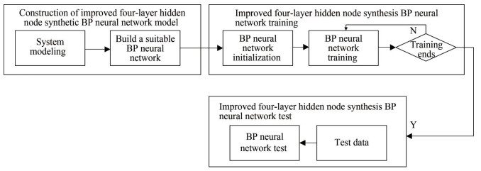Figure  2  Flowchart of the improved four-layer hidden node synthetic BP neural network algorithm

Download: Full-Size Img

3   Multi-objective ship route induction model

3.1   Ship traffic flow theory

This research is based on ship traffic flow theory, which provides important data support for subsequent ship route induction. This theory is a model and method system that studies the variation of traffic flow over time and space, mainly including the basic theories of traffic planning and traffic control. In the context of ship traffic flow theory, some scholars have focused on the safety issues of ships by combining wave theory (Shao et al., 2002) and queuing theory (Chen et al., 2001), but a systematic theoretical system has not been formed. A relationship model between the three parameters of traffic flow characteristics (flow, speed, and density) has been proposed in the literature (Zhu, 2010). The flow–speed relationship is represented by Equation (9).

where q is the flow of the ship flow, Vessels/h; q_f is the flow of ships in the free-flow state, Vessels/h; q_max is the maximum vessel flow in the channel, Vessels/h; v is the speed of the ship, km/h; v_f is the free-flow speed, km/h; ρ for ship flow density, Vessels/km; ρ_f is the maximum vessel density in a channel under free flow, Vessels/km; ρ_j is the blocking density, Vessels/km; and k is the wave velocity coefficient, 0 ≤ k ≤ 1.

3.2   Ship route induction objectives

Traditional ship route induction usually focuses on a single induction target, such as analyzing factors like navigation time, distance, and costs. However, this approach of considering only one factor in ship route induction does not align with the "dual-carbon" strategy proposed by China in recent years. Therefore, this study presents a multi-objective ship route induction method based on existing research in the field. This method introduces a combined route impedance function during the ship route induction process. The study proposes a comprehensive model of the route impedance function, which takes into account five variables: navigation time, distance, costs, fuel consumption, and carbon emissions. Each of these five influencing factors is analyzed separately below.

3.2.1   Relationship between fuel consumption and fuel costs and carbon emissions

The cost of ship operation includes fuel expenses. When ships navigate within Bohai Bay, where the surrounding environment is relatively stable, and the impact of wind and waves can be negligible, the fuel consumption for a given ship's load depends on the distance, speed, and time of navigation. The navigation time is directly related to the distance and speed of the voyage. The principle of ship fuel consumption is that the ship's main engine consumes fuel to drive the propeller's rotation. When the ship's load remains constant, and it travels at a constant speed, the effective thrust exerted on the ship's hull balances the total resistance it experiences. This study utilizes the following formula to calculate fuel consumption:

where F (R) is the total fuel consumption, t_i is the sailing time of the vessel in the ith leg of the voyage, FCPH_i (v) is the fuel consumption per unit time of the ship, R_iw is water surface and air resistance, P_S is the host power, P_E is the effective power of the ship, S_FOC is the fuel consumption rate, η_S is shafting efficiency, η_R is the relative rotational efficiency, η_O is the efficiency of open water slurry, and η_H is the hull efficiency.

After obtaining the fuel consumption, the fuel cost can be obtained as follows:

where F is the total fuel cost, and p is the unit price of fuel. From Equation (14), fuel cost is directly and linearly proportional to fuel consumption.

Below is an analysis of carbon dioxide emissions indicators.

The Energy Efficiency Operational Indicator (EEOI) for shipping refers to the carbon dioxide emissions generated per unit of transportation work by a vessel. The calculation formula for EEOI is as follows:

where F (R)_i is the fuel consumption of the ship in the ith leg, C_F is the conversion factor between the amount of fuel per unit and the amount of carbon dioxide, M_i is the deadweight of the ship in the first route segment (tons), D_i is the operating distance of the ship in the first leg of the voyage (nautical miles).

From Equation (15), the CO₂ emissions produced by the ship transporting M tons of cargo on the ith route segment D nautical mile is F (R)_i·C_F, so the CO₂ emissions generated by the transportation of a rated cargo load over a certain distance on a specific shipping route are directly proportional to the fuel consumption during that period. Based on the previous analysis, both fuel costs and CO₂ emissions are linearly related to fuel consumption. In the subsequent multi-objective optimization process, reducing fuel consumption is necessary to achieve the goals of reducing operating costs and carbon emissions.

3.2.2   Relationship between sailing distance, sailing time, and fuel consumption

Owing to the variability of sailing speed depending on the traffic flow, the fuel consumption per unit time increases with high speeds. However, the sailing time may be reduced. Therefore, the relationship between sailing time and fuel consumption cannot be simply viewed as directly proportional or inversely proportional. Similarly, the distance of the voyage cannot directly determine the fuel consumption. Hence, the sailing distance, sailing time, and fuel consumption are the three factors that should be optimized in combination in this context.

3.3   Joint road resistance function

The road resistance function, also known as the resistance function, is a mathematical expression that quantifies the road impedance. The resistance function can comprehensively reflect the relationship between travel time and traffic conditions (e.g., traffic speed, flow, and density) as well as road conditions (e.g., road width, geometric shape, and road type). This function is the definition of the land transportation resistance function. In this context, the joint resistance function is actually a reflection of the relationship between the comprehensive road weighting and the traffic conditions in the maritime route network.

Based on the analysis mentioned above, this study aims to optimize three objectives: minimizing sailing distance, sailing time, and fuel consumption. Previous experience in solving multi-objective optimization problems demonstrates that finding a solution that satisfies all optimization objectives is rare. Instead, we can find relatively optimal solutions. In this study, a method is employed to reduce the dimensionality of the objective functions to address the multiobjective planning problem.

First, the dimensionless processing of each objective is performed to unify the different measurement standards. Then, the weights are assigned to the objectives according to the importance of each objective for downgrading the multi-objective function problem into a single objective function problem. The comprehensive cost function analysis highlighted that the units of each indicator in the index system are different. The relevant evaluation calculation cannot be performed, so the concept of dimensionless must be introduced to carry out the unit normalization (Ahmed et al., 2021). The computational problems caused by the unit are not considered, which in turn is transformed into a pure numerical calculation to facilitate the unified evaluation of different indicator units. The navigation program column {L₁, L₂, …, L_N}, flight time sequence {T₁, T₂, …, T_N}, and energy consumption sequence {E₁, E₂, …, E_N} are standardized.

The new sequence is obtained, i.e., {y₁, y₂, …, y_n} ∈ [0, 1], and it is dimensionless. Standardizing the factors influencing the comprehensive cost route ensures that they are within the same numerical range. Subsequently, weighted calculations are performed to obtain the comprehensive cost value for each route segment. Finally, the route with the minimum value of the comprehensive cost function is selected.

Based on the above analysis, the comprehensive road resistance function can be expressed as

where F_i (v) is the combined right-of-way value for the ith leg; l_i is the dimensionless range value of the ith route segment; t_i is the dimensionless sailing time value of the ith route segment; e_i is the dimensionless energy consumption value of the ith route segment; w_L, w_T, and w_E are the proportion of range, flight time, and energy consumption, respectively; and w_L + w_T + w_E = 1. Based on the different emphasis of optimization objectives, the weights can be adjusted accordingly. In this study, the same weight is assigned to each indicator for route induction.

3.4   Induction model establishment and solution

We set the map to G = (V, E) the shortest path r from vertices s.

represents the weight of this edge i; x_i represents the edge that is selected to pass; and x_wv indicates whether to choose to pass the w → v side.

The shortest path problem is about finding the shortest route from a starting point to a destination in a network (Lv et al., 2022). Algorithms for solving the shortest path problem include Dijkstra's algorithm and Floyd's algorithm. Dijkstra's algorithm can find the shortest path from the origin to any node in the network, whereas Floyd's algorithm is more widely applicable because it can compute the shortest paths between any two points in the network. This study is focused on inducing complete shipping routes, so the improved Dijkstra's algorithm is chosen to solve the problem. To apply Dijkstra's algorithm to solve the multi-objective ship route induction problem, the shortterm traffic flow prediction from previous chapters and the joint impedance values calculated based on ship traffic flow theory should be combined to assign weights to the route network. The route with the lowest comprehensive navigation cost for ships passing through the induction area is determined.

The specific operation steps of Dijkstra's algorithm are as follows:

1) Label vertex v1 with P, d (v1)= 0 and v_j (j = 2, 3, …, n) with T, d (v_j) = l_1j.

2) Take the smallest of all labels, for example, d (v_j0) = l_1j0, The T designation of v_j0 is changed to the P designation, and recalculate the label T for each other vertex with T. The smaller of the T designators d (v_j) and d (v_j0) + l_{j0 j} of vertex v_j is chosen as the new T designator of v_j.

3) Repeat the above steps until the target vertex is changed to P.

This study aims to achieve the effect of dynamic ship route induction, which requires improvements to the existing Dijkstra algorithm, that is, changing the arc weights of unlabeled nodes in the route network. As mentioned earlier, the predicted ship traffic is in different time periods, and the changes in ship traffic directly lead to changes in the arc weights in the road network, which in turn affect the choice of nodes by the algorithm. Therefore, when a ship passes through each node, which time period the node is in at that moment must be determined. If it exceeds the time period in which the originating time is located, the traffic flow on each route segment in the route network must be updated, and the weights of the route segments should be recalculated, repeating the steps until the ship reaches its destination.

4   Case study

4.1   Flow forecasting

To test the applicability of the above model, the hourly ship traffic flow in the bay from April 3 to May 5, 2023, at several sections from 0:00 to 24:00, was studied. The ship traffic flow refers to the upstream and downstream ship traffic flow through the section. Historical data were collected through the shipxy. Based on the traffic flow data from April 3 to May 5, the traffic flow at each section on May 6 was predicted. The information collection interface is shown in Figure 3.

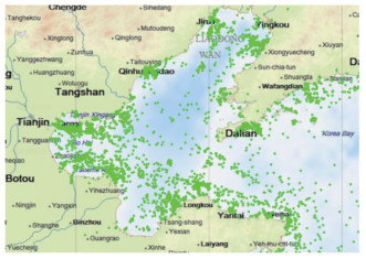Figure  3  Information collection map of a bay

Download: Full-Size Img

For the sake of research convenience, a simplified vector diagram of ship routes within a bay is presented here. The ship route vector diagram is based on the consideration of the driver's driving habits and the fitting of historical ship route tracks. The ship route vector diagram is shown in Figure 4. Points 1, 2, 3, 4, 7, 8, 14, 15, 21, 22, 23, 24, and 25 represent various ports within the induced area.

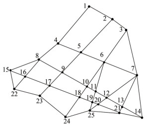Figure  4  Vector diagram of ship routes in a certain bay

Download: Full-Size Img

Through the AIS ship information monitoring system, the statistics of ship traffic flow are shown in Table 1. This route network includes 12 routes (1-2-3-7-14, 4-5-6-7, 8-9- 10-11-12-13-14, 15-16-17-18-19-20-21-14, 15-22-23-24- 25-21, 1-4-8-15, 8-16-22, 2-5-9-17-23, 3-6-10-18-24, 6-11- 19-25, 7-12-20-25, and 7-13-21). Owing to the large number of route sections involved, only the ship traffic flow statistics of some route sections are given. Table 1 shows the ship traffic flow statistics of each route section of Route 1-2-3-7-14 on a certain day. The statistical routes are shown in Figure 5.

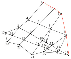Figure  5  Statistical route chart

Download: Full-Size Img

Running the compiled program can obtain the learning curve, neural network learning diagram, and prediction results. The learning curve of the network is shown in Figure 6. In the figure, the error of the network training is very small, and it reaches the target value. The neural network learning diagram is shown in Figure 7, and the network's fitting performance gradually improves with the increase of the sample number.

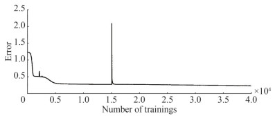Figure  6  Network training results

Download: Full-Size Img

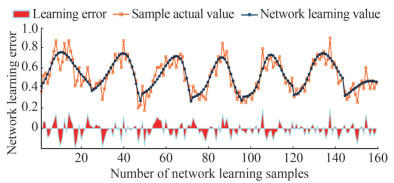Figure  7  Neural network learning schematic

Download: Full-Size Img

According to the above method, the flow prediction values for each cross section can be obtained sequentially. The flow prediction values for sections 1-2-3-7-14 are shown in Table 2.

4.2   Model solving

We use the ship flow data from the AIS system and combine it with the short-term traffic flow prediction method proposed in this study to predict the ship flow for a future time interval. Through the above prediction method, the flow prediction values for each section of the experimental route network on May 6, 2023 can be obtained. The prediction results are combined with the ship traffic flow theory introduced in the second part of this paper to calculate the recommended sailing speed for each section of each route. Based on these recommended sailing speeds, we can calculate the travel time, fuel consumption, and other indicators. Based on these indicators, we calculate the integrated right-of-way value set as the right-of-way for each route, as shown in Table 3. Finally, the route with the lowest integrated right-of-way value is induced for the ship.

The experimental study optimizes the dynamic path of ships from port 1 to port 25 based on the guiding target. We assume that the ships enter the area at 7:00 (UTC+8) and update the ship network route for each arrival at a node, re-planning the voyage route for the ships. The previously traveled region is used as the historical trail and is no longer re-searched. As shown in Figure 4, the first planned route for the ships is 1-2-3-6-10-11-12-20-25 (as shown in Figure 8), and the second planned route for the ships is 1-2-3-6-11-12-20-25 (as shown in Figure 9). The two planned routes are clearly different. Following the above experimental steps, the iteration update is continued until the ships reach the destination. The network route updates are shown in Figure 10 to Figure 15.

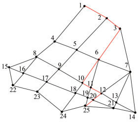Figure  8  Route map under static road network information

Download: Full-Size Img

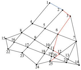Figure  9  Route diagram after the initial weight update

Download: Full-Size Img

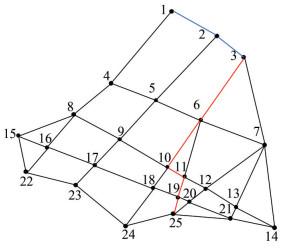Figure  10  Route diagram after the second weight update

Download: Full-Size Img

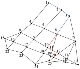Figure  11  Route diagram after the third weight update

Download: Full-Size Img

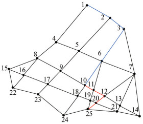Figure  12  Route diagram after the fourth update of weights

Download: Full-Size Img

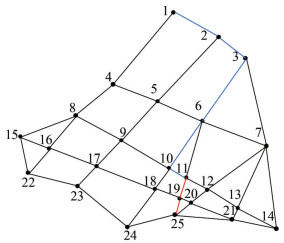Figure  13  Route chart after the fifth update of weights

Download: Full-Size Img

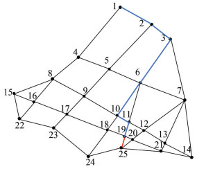Figure  14  Route diagram after the 6th update of weights

Download: Full-Size Img

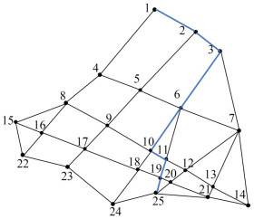Figure  15  Route map under dynamic road network information

Download: Full-Size Img

The experimental results can be divided into two parts: static ship route induction and dynamic ship route induction. As shown in Figure 16, for the first planned route (static ship route induction) 1-2-3-6-10-11-12-20-25, the total integrated right-of-way of this path is 1.657. For the final planned route (dynamic ship route induction) 1-2-3-6- 10-11-19-25, the integrated right-of-way value of this path is 1.3663, which is 17.55% less than the static route induction. The static induction leads to a travel distance of 260 nautical miles, travel time of 20.6 h, and fuel consumption of 10.4 t, while the dynamic induction leads to a travel distance of 248 nautical miles, travel time of 19.31 h, and fuel consumption of 9.92 t, reducing by 4.6%, 6.26%, and 4.62%, respectively. The results show that the dynamic ship route induction performs better than the static ship route induction for each guiding target, highlighting the reliability and practical significance of the method. In particular, it plays an important role in addressing energy conservation and reducing emissions. By conducting in-depth research on the routes of ships in the bay, questions such as route selection, changes in traffic flow, and route planning can be explored. This research is of great management significance for relevant stakeholders such as government departments, port operators, and shipping companies. Furthermore, such research can help formulate effective bay management strategies and navigation rules.

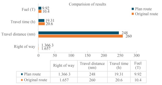Figure  16  Comparative analysis of induction results

Download: Full-Size Img

5   Concluding remarks

In this study, a dynamic ship route induction method based on predictive data and multiple variable factors is proposed by combining the idea of dynamic induction of land traffic and the actual situation of sea traffic. The method can continuously update route planning based on real-time traffic flow data and adjust the weights according to the importance of different induced objectives, which is highly flexible and effective. In route induction, the method also considers the carbon emission factor, which reduces the carbon emission under the premise of ensuring navigation efficiency. It is also in line with the current direction of the shipping industry, which needs to be adjusted. The experimental analysis results show that the dynamic induction method is better than static route planning and can obtain the route planning with the lowest comprehensive cost and in line with people's expectations, which has certain practical value and engineering significance. However, the method has certain limitations. In the case of a relatively stable offshore sea area, the method can provide the best traveling route for the ship in a short time. If the ship is traveling in the oceanic sea area and the sea condition is complicated and changeable, the induction effect of this method is unsatisfactory. Overall, the dynamic ship route induction method has great potential to improve the navigation efficiency of ships and the sustainable development of maritime transport, and it has become an important development direction in the field of navigation.