1   Introduction

Ship thrust in ice is influenced by two factors: total ice resistance and the pulling performance of the propulsion system. In recent years, significant progress has been made in experimental and calculation techniques to determine ice resistance. The efforts of ITTC ice experts have led to detailed recommendations for model tests in ice basins with nonpropelled (ITTC, 2017a) and propelled models (ITTC, 2017b). With these guidelines in hand, the ice resistance of icebreakers and ice-going vessels under design can be accurately predicted.

Modern methods with high prediction potential are used to calculate ice resistance (Lindqvist, 1989; Su et al., 2010; Su et al., 2011; Tan et al., 2014; Valanto, 2009). These references, along with numerous other studies, enable the determination of ice resistance with sufficient accuracy for design purposes, particularly under close-to-limit ice conditions.

Research on the operation of icebreaker propulsion systems in the vast majority of cases has focused on propeller interaction with ice. In this field, significant advancements have ensured the strength of the propulsion system, including azimuth thrusters, and provided insights into the dynamics of the propeller–shafting–engine system under ice loads (Andryushin et al., 2013; Dobrodeev et al., 2017; Ikonen et al., 2015). At present, the mathematical modeling of propeller interaction with ice is rapidly developing. For example, Chao et al. (2017) considered variations in thrust coefficient K_T and torque coefficient K_Q during these processes. However, the hydrodynamic issues of icebreaker propellers have not been adequately studied. Specific hydrodynamic problems of icebreaker propellers, such as cavitation, were discussed solely by Alekseev et al. (1993) and Walker et al. (1994).

The issues of propeller/hull interaction for ships in ice were discussed in the 1980s by Juurmaa and Segercrantz (1981) and by the ITTC ice committee (Schwarz et al., 1987) during the analysis of self-propelled model test results obtained for an R-class icebreaker in various basins around the world. Leiviskä (2003) analyzed the propeller/hull interaction coefficients of a ship with steerable gondola (pod) sailing ahead and astern in ice. The experimental method for determining model ice resistance adopted in the HSVA ice basin (2011) can determine thrust deduction coefficient values. However, the authors are not aware of any publication by researchers in this basin where the obtained results were generalized. Luo et al. (2018) described the method of investigating the propeller wake model of a single-screw heavy-tonnage ice-class vessel with ice on the underwater hull surface. Therefore, the issues of propeller/hull interaction in ice conditions have not received adequate attention, although these concerns directly relate to the calculation of ship thrust characteristics in ice.

Traditional methods for determining thrust in ship theory encounter technical difficulties related to defining propeller/hull interaction coefficients (Kanevskii et al., 2017). The effective thrust developed by the propulsion system can be easily calculated and experimentally determined under bollard pull conditions. Furthermore, effective thrust can be calculated at sufficiently high ship speeds. Consequently, different approximation formulas have been used to determine the effective thrust of icebreakers and icegoing vessels in ice. For example, in Su et al. (2010), the net thrust is approximated by a square parabola:

In this formula, T_E^boll represents the net thrust of the propulsion system in bollard pull conditions, and V_ow denotes the maximum ship speed in open water at a given power level. The approximation factors in this formula are the same for any vessel.

Accurately calculating the thrust characteristics of a ship's propulsion system is challenging, which is a serious obstacle to determining full-scale ship ice resistance. This calculation can be achieved only by measuring the thrust of the ship's propulsion system during sea trials and determining the thrust deduction coefficient based on model test data (Sodhi et al., 2001; Spencer and Jones, 2001). The relationship between full-scale and model experiments is frequently examined by comparing power consumption (Jones and Lau, 2006; Lau, 2015).

Typically, icebreakers and ice-going vessels are multishaft ships to absorb greater power. This design feature adds complexity to calculations because of the need for special-purpose procedures (Kanevskii et al., 2020).

Currently, the model test data obtained in ice basins offers a straightforward method for assessing only the limiting ice capability of icebreakers and ice-going vessels, specifically the maximum thickness of ice through which the ship can continuously move at the maximum power of its main engines with a minimum stable speed. Evaluating ice performance in a wider range is possible but requires numerous overload tests, which are typically not conducted. Therefore, information on performance in ice is lacking for most projects. Consequently, the thrust, torque, number of revolutions, and efficiency of propellers in a wide range of ship operating modes in ice cannot be accurately predicted. Considering this lack of information, assessing the efficiency and optimizing the performance of icebreakers and ice-going vessels are impossible. In this context, predicting the performance of icebreakers in ice for the full range of operational conditions is a serious problem today. This work proposes a method for calculating the propulsion performance and thrust characteristics of a ship operating in ice conditions. The initial data for the method are provided by model tests in hydrodynamic and ice basins, including towing resistance in open water and ice, hydrodynamic characteristics of propellers in open water, and propeller/hull interaction coefficients. The proposed method for evaluating ship propulsion performance in ice is suitable for single- and multi-shaft vessels equipped with propellers and propulsion pods.

2   Hydrodynamics of propeller/hull interaction in ice

2.1   Problems of traditional approaches in evaluating ship performance

A conventional approach to estimating the propulsion performance of a ship in open water is based on model tests in towing tanks. These tests are used to determine water resistance versus model speed, hydrodynamic characteristics of an isolated propeller, and propeller/model hull interaction coefficients. The latter are identified by comparing the hydrodynamic characteristics of open-water and behind-hull propellers. Three classical coefficients of interaction for a given speed are determined following relevant procedures mentioned in ITTC (2017c): w—wake fraction, t—thrust deduction coefficient, and η_R—relative rotative efficiency.

Wake fraction w is given as

where J_o, J are the propeller advance coefficients in open water and behind the hull, respectively; K_To, K_T are the propeller thrust coefficients in open water and behind the hull, respectively.

Eq. (2) outlines the relationships between propeller advance coefficients in open water and behind the hull. According to Eq. (2), the wake fraction w is determined at identical thrust in open water and behind the hull. In this context, unlike ITTC (2017c), the subscript "о" denotes "open water".

Relative rotative efficiency η_R is defined by

The open-water torque coefficient in Eq. (3) is determined by the same open-water advance coefficient, which is calculated using the wake fraction.

The thrust deduction coefficient t is calculated using the formula:

In Eq. (4), the following symbols are used:

— T_M represents the total thrust of a ship model propeller; here, subscript M means ship model;

— F_D denotes an additional towing force due to the difference in the model and full-scale resistance coefficients;

— R_TM refers to the towing resistance of the ship model.

When Formulas (2) – (4) are applied at small advance coefficients, difficulties may arise in defining the wake fraction w. The dependence of hydrodynamic coefficients of thrust and torque on the advance coefficient in open water and behind the hull has specific features. At small advance coefficients J ≤ 0.2 ÷ 0.3, the following relations are found: K_T(J) < K_To (J_o) and K_Q(J) < K_Qo (J_o). In using Formula (2), the wake fraction value becomes negative and tends to infinity as J → 0. Figure 1 illustrates the hydrodynamic propeller characteristics of the R-class icebreaker Franklin, as documented by Michailidis and Murdey (1981). This figure clearly demonstrates the aforementioned specific feature.

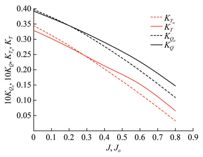Figure  1  Hydrodynamic propeller characteristics of the R-class icebreaker Franklin

Download: Full-Size Img

When Formula (2) is applied to the hydrodynamic propeller characteristics of the R-class icebreaker Franklin, it yields negative wake fractions that tend to minus infinity as the advance coefficient J approaches bollard pull conditions. Figure 2 shows the wake fraction versus advance coefficient, which is calculated using the data in Figure 1.

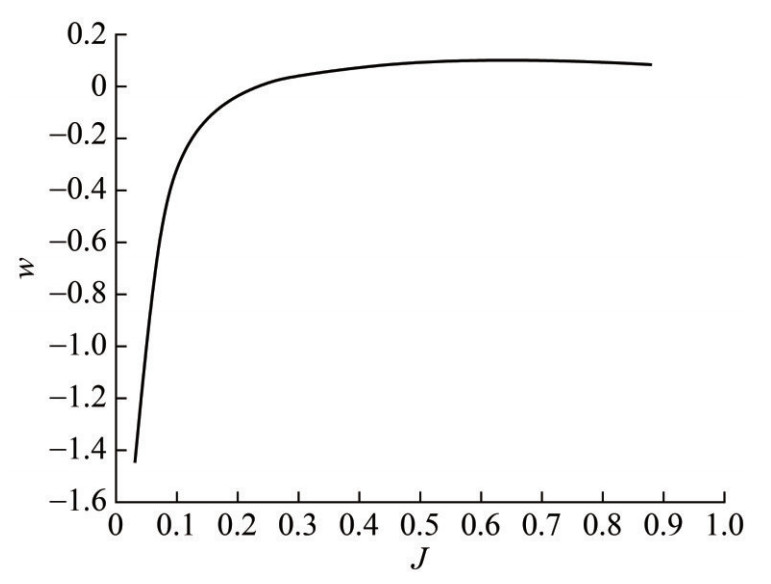Figure  2  Wake fraction versus advance coefficient for the propeller of the R-class icebreaker Franklin

Download: Full-Size Img

The situation depicted in Figure 1 is common. According to the authors' experience, up to 90% of the models tested in hydrodynamic basins at the Krylov State Research Centre (St. Petersburg, Russian) exhibit this abnormality. The icebreaker Vladivostok, which is discussed below, is an example in this case. Hydrodynamic laboratories typically do not publish data on the operation of propulsion systems behind model hulls, which causes difficulty in providing a longer list of ships based on the literature.

This issue is the primary obstacle to applying traditional methods for calculating the propulsion performance of a ship operating at small advance coefficients. However, small advance coefficients are typical for ships moving in ice.

2.2   Alternative system of interaction coefficients

The Krylov State Research Centre has developed an alternative system of coefficients to characterize propeller/hull interaction when the propeller operates near bollard pull conditions to address the aforementioned challenges (Kanevskii and Klubnichkin, 2017). As in the traditional system, this alternative system of coefficients includes three coefficients for a given ship speed: the coefficient of hull influence on thrust i_TB, the coefficient of hull influence on torque i_QB, and the thrust deduction coefficient t. This suggested system of coefficients is universal and applicable in all scenarios where the traditional system is applied.

The propeller/hull interaction coefficients in the alternative system are derived from experimental data obtained in hydrodynamic test basins. These coefficients are determined from experimental data at a specific advance coefficient J. For this purpose, the open-water thrust and torque coefficients K_To, K_Qo of propellers are obtained from experimental plots. The interaction coefficients itself are defined by the following relations at J = J_о:

— coefficient of hull influence on thrust:

— coefficient of hull influence on torque:

— thrust deduction coefficient:

The procedure for determining the thrust deduction coefficient remains the same as in the traditional system. Figure 3 illustrates the alternative system for defining the interaction coefficient.

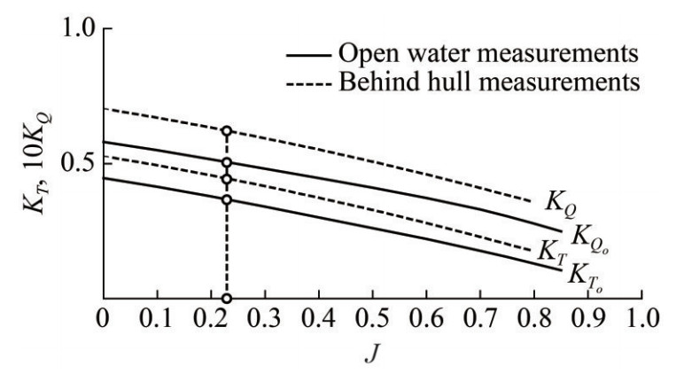Figure  3  Illustration of the alternative system for propeller/hull interaction coefficients

Download: Full-Size Img

A distinctive feature of the alternative system is the flow velocities around the propeller in open water and behind the model hull are equal, which leads to equal advance coefficients; however, the propeller thrusts are not the same.

Figure 4 shows the alternative system for the interaction coefficients of the propeller of the R-class icebreaker Franklin, as documented by Michailidis and Murdey (1981).

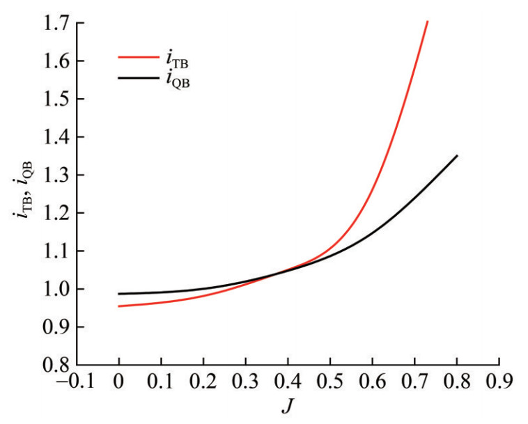Figure  4  Interaction coefficients i_TB and i_QB versus propeller advance coefficient for the R-class icebreaker Franklin: an alternative system (Michailidis and Murdey, 1981)

Download: Full-Size Img

2.3   Method for experimental determination of alternative interaction coefficients

The interaction coefficients of the alternative system, as previously mentioned, can be derived from the same propulsion tests used to determine traditional interaction coefficients. However, identifying these coefficients in the advance coefficient range J < 0.3, which is typical of ships in ice conditions, requires a substantial set of experiments. In this case, towed propulsion tests are conducted with a self-propelled model rigidly connected to a towing carriage. These experiments are performed at a fixed speed of the model with variations in propeller revolutions (overload tests). In this case, the model is subjected to a braking force from the towing carriage F_D, which simulates ice resistance.

Such investigations have been conducted in propulsion studies of R-class icebreakers (Michailidis and Murdey, 1981) and the icebreaker Healy (Jones and Lau, 2006; Jones, 2004). However, these explorations did not apply the alternative system of interaction coefficients. Using the traditional system, only the thrust deduction coefficient t could be determined by overload tests. In addition, the experimental results occupy a significant area on the graph of thrust deduction coefficient t versus icebreaker model speed. Notably, when the overload test data are presented as thrust deduction coefficient versus advance coefficient t = t (J), the results align in a single line (Kanevskii and Klubnichkin, 2017).

At the Krylov Centre, overload tests with alternative interaction coefficients are conducted for each model of icebreakers and ice-going vessels. In self-propulsion tests, the propeller revolutions are constant and selected based on the given power. The speed of the model ship varies from zero to full speed. In this case, presenting the overload test results versus the advance coefficient J is inconvenient for propulsion estimates because the relation for determining the advance coefficient includes propeller revolutions:

where V is the ship speed, n denotes the number of propeller revolutions, and D represents the propeller diameter.

The most convenient way of presenting the overload test results is versus parameter K_DE, which is defined as

where K_E is the effective thrust of the propeller, which is defined as

where ρ refers to water density, and T_E is the propeller effective thrust determined in overload tests by the following formula:

Eq. (11) is derived from Eq. (4) of ITTC (2017c).

The parameter K_DE is useful for presenting overload test data because it is a non-dimensional parameter that does not contain propeller revolution and is not zero in bollard pull conditions. Notably, the K_DE value can be estimated using dimensional parameters by the following formula:

In Formula (12), Z_P is the number of propellers, and Z_P = 1 or 2. Formula (12) is also applicable for Z_P > 2 if the diameters of the propellers are the same. The process of determining the parameter K_DE for different propeller diameters is described in Kanevsky et al. (2020).

As an example, Figure 5 presents alternative interaction coefficients versus K_DE for an ice-going vessel.

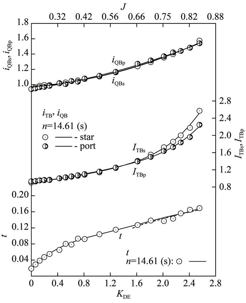Figure  5  Interaction coefficients t, i_TB, and i_QB of the alternative system for an ice-going vessel

Download: Full-Size Img

At the top of this figure, the values of the advance coefficient J are shown. In overload tests, the non-dimensional parameters J and K_DE are related by the following dependence.

Notably, after self-propelled model tests, three values are obtained at a given speed: w—wake fraction, t—thrust deduction coefficient, and η_R—relative rotative efficiency.

Overload tests provide three dependencies of alternative coefficients on the parameter K_DE : i_TB (K_DE)—coefficient of hull influence on thrust, i_QB(K_DE)—coefficient of hull influence on torque, and t (K_DE)—thrust deduction coefficient.

This situation is not accidental and is related to the fact that the towing force F_D varies during overload tests at a given speed V. An icebreaker can move at the same speed in different ice conditions, such as in level or broken ice. The ship speed in ice conditions does not determine the ice resistance. Naturally, the power consumed by the icebreaker depends on the ice resistance.

2.4   Prediction of ship propulsion performance in ice conditions

The prediction of ship propulsion performance in ice conditions follows the recommendations of ITTC (2017c). The key difference between the suggested procedure and the generally accepted techniques is the introduction of alternative interaction coefficients.

The dataset for predicting ship propulsion in ice includes ship speed V_S, where the subscript S refers to the ship; wetted surface of the ship S_S; propeller diameter D_S; number of propulsive units Z_P = 1 or 2; water density in full-scale conditions ρ_S; electrо-mechanical efficiency η_SH; functions of hydrodynamic characteristics of open-water propellers designed for the ship K_ToS(J_S), K_QoS(J_S), which are scaled to full size (ITTC, 2017c); and alternative interaction coefficients as a function of the parameter K_DE. An alternative interaction coefficient includes i_TB (K_DE)—coefficient of hull influence on thrust, i_QB (K_DE)—coefficient of hull influence on torque, t (K_DE)—thrust deduction coefficient, and total ice resistance of the ship R_IS.

The prediction of ship propulsion in ice starts with estimating the parameter K_DE, which is defined as

The value of the K_DE parameter is used to determine i_TB, i_QB, and t.

The prediction of ship propulsion performance in ice-free water is based on the relation $ \frac{K_{\mathrm{T}_o \mathrm{S}}}{J_S^2}=f\left(J_S\right)$. This function can be readily derived using the hydrodynamic characteristics of full-scale propellers in open water K_ToS(J_S). The same function is utilized for predicting the ice performance of ships.

The 1978 ITTC Performance Prediction Method uses the total resistance coefficient in ice-free water C_TS. To reduce the difference between the proposed procedure and the ITTC method, we introduce the total resistance coefficient:

where S_S is the wetted surface of the ship hull. Unlike in ice-free water, the total ice resistance coefficient is assumed to be free of scale effects at slow speeds V_S < 7 knots, and its value is the same for the ship and its model:

Then, the expression for $ \frac{K_{\mathrm{T}_o \mathrm{S}}}{J_S^2}$ using the alternative interaction coefficients can be re-written as follows:

The value of $ \frac{K_{\mathrm{T}_{{o}} \mathrm{S}}}{J_S^2}$calculated from Eq. (16) allows for the determination of the advance coefficient at given ship speeds and ice conditions J_TS and the propeller torque coefficient K_QoTS.

A distinctive feature of the alternative interaction coefficients is that J_s = J_o; that is, all coefficients are determined at a constant advance coefficient. Consequently, the number of revolutions is defined as

Power consumed by each propeller:

Propeller thrust:

Propeller torque:

Effective power:

Hydrodynamic efficiency:

Hull efficiency:

Relative rotative efficiency:

Efficiency:

Here, η_SH is the electromechanical efficiency, and η_S refers to the open-water propeller efficiency:

3   Results and discussion

3.1   Case study

The diesel-electric icebreaker Vladivostok, with project number 21900М, was selected for the case study. The icebreaker was constructed in 2015 by Vyborg Shipyard. This double-decker vessel features two 360° azimuth thrusters with a power of 2.9 МW. The ship was designed for the Icebreaker 6 class by the Russian Maritime Register of Shipping, as shown in Figure 6.

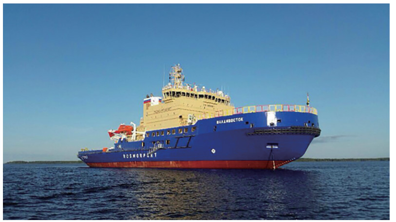Figure  6  Icebreaker Vladivostok, Pr. 21900М

Download: Full-Size Img

During the design phase, the Krylov Centre conducted a full cycle of tests, including hydrodynamic and ice basin tests. Based on the self-propulsion tests in the hydrodynamic tank, the functions for the alternative system of propeller/hull interaction coefficients were determined. These functions are presented in Figure 7.

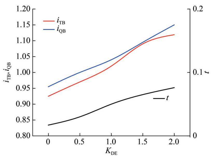Figure  7  Interaction coefficients t, i_TB, and i_QB of the alternative system for the icebreaker Vladivostok

Download: Full-Size Img

The propulsion performance of the icebreaker in 1.5 m-thick level ice at a speed of 3.0 knots was calculated using Eqs. (13)–(26).

The initial data inputs were as follows:

— ship wetted surface S_S = 3 400 m²;

— propeller diameter D_S = 4.5 m;

— number of propulsors Z_P = 2;

— water density in full-scale ρ_S = 1 025 kg/m³;

— electro-mechanical efficiency η_SH = 0.95;

— hydrodynamics characteristics of 2.9 МW azimuth thrusters in open water K_ToS (J_S), K_QoS (J_S);

— alternative interaction coefficients versus K_DE;

— total ice resistance of ship R_IS = 1 460 kN.

The calculations yield the following results:

— icebreaker speed V_S = 1.543 m/s;

— K_DE = 0.260;

— coefficient of hull influence on thrust i_TB = 0.949;

— coefficient of hull influence on torque i_QB = 0.980;

— thrust deduction coefficient t = 0.022;

— total ice resistance coefficient C_IS =0.352;

— $ \frac{K_{\mathrm{T}_{{o}} \mathrm{S}}}{J_S^2}$ = 15.942;

— advance coefficient J_TS = 0.155;

— thrust coefficient K_ToTS = 0.383;

— torque coefficient K_QoTS = 0.057 5;

— number of propeller revolutions n_S = 2.213 1/s = 132.6 RPM;

— power consumed by each propeller P_DS = 7 224.8 kW;

— thrust of azimuth thruster pod T_S = 746 kN;

— propeller torque Q_S = 520.3 kN⋅m;

— effective power P_E = 2 253.2 kW;

— hydrodynamic efficiency η_D = 0.156;

— hull efficiency η_H = 0.947;

— efficiency η = 0.148;

— azimuth thruster efficiency in open water η_S = 0.164. The analysis results of level ice trial data for the Vladivostok and Novorossiysk icebreakers are presented in Tables 1 and 2 below (Kostylev et al., 2016; Lopashev et al., 2017).

The calculation results for propeller RPMs, as shown in Tables 1 and 2 and Figure 8, reveal a strong correlation with the ice trial data. The deviations between these results are likely due to the absence of the ice shroud (ice pieces submerged by the underwater surface of the icebreaker hull) and the lack of ice on the water surface during self-propulsion tests.

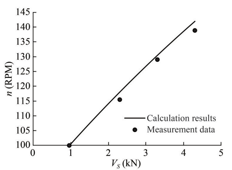Figure  8  Propeller RPM n versus speed V_S of the Novorossiysk icebreaker during ice trials

Download: Full-Size Img

The calculation results for ice resistance shown in Tables 1 and 2 were extrapolated to the ice thickness of 1.5 m and a standard bending strength of 500 kPa. The extrapolation to the ice thickness of h was conducted according to the recommendations of ITTC (2017a) and Jochmann et al. (2014) using the following relationship:

where R_I represents the ice resistance, and h refers to ice thickness.

The extrapolation of the ice trial data for the Vladivostok icebreaker to the standard bending strength was conducted according to the recommendations of ITTC (2017a) and Jochmann et al. (2014) using the following relationship:

Here, a indicates the portion of the ice resistance due to forces dependent on the bending strength of the ice, σ_f represents the bending strength, meas denotes the measured value, and target refers to the required value.

Calculations of resistance to the icebreaker, according to Eqs. (27)–(28), moving in a 1.5 m-thick level ice field with a standard bending strength of 500 kPa, are shown in Figure 9 below.

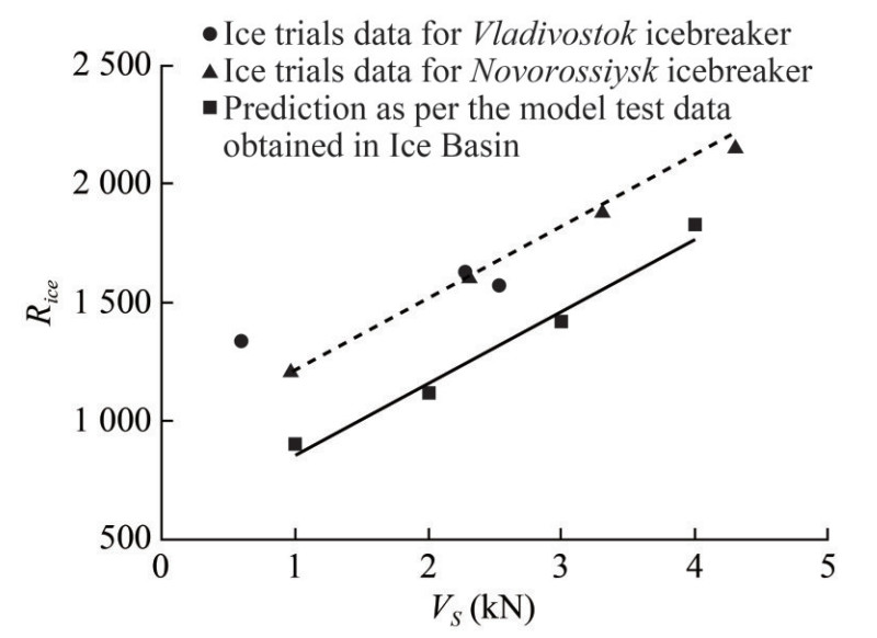Figure  9  Ice resistance R_ice for the Vladivostok icebreaker in a 1.5 m-thick ice field (bending strength of 500 kPa)

Download: Full-Size Img

These icebreakers, as per the model test data obtained in the Ice Basin, show predictions that qualitatively align with the results of full-scale trials. Discrepancies may arise because the calculation ignored the effect of the ice shroud and the ice on the water surface during self-propulsion tests on the hydrodynamic parameters of propeller/hull interaction.

Figure 10 compares the dependence of the icebreaker effective thrust calculated by the proposed method and Formula (1) at V_ow = 17.4 knots. This graph clearly indicates an error in Formula (1) compared with the suggested method.

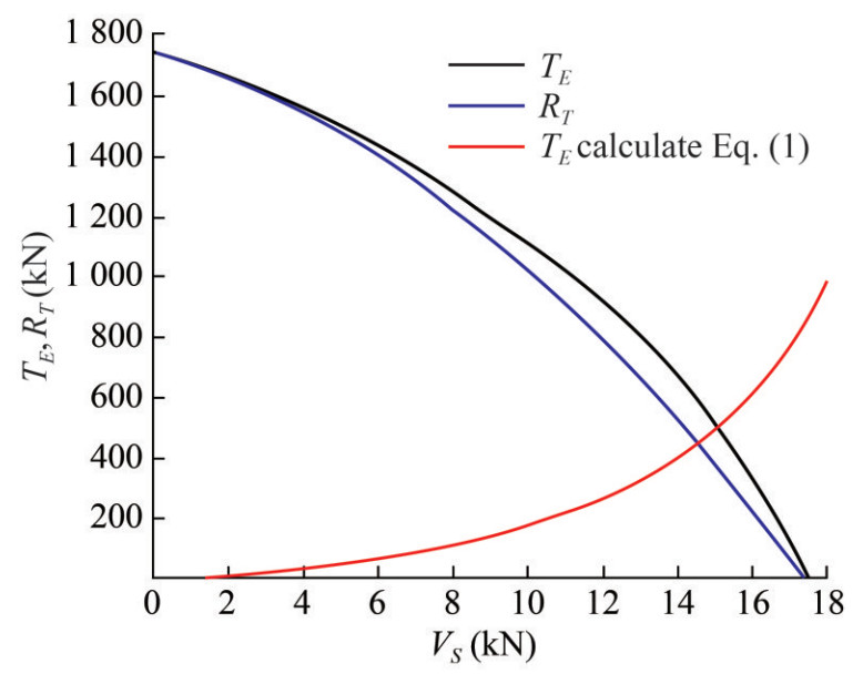Figure  10  Comparison of the net thrust characteristics of the icebreaker calculated by the suggested method and Formula (1)

Download: Full-Size Img

3.2   Ice interaction coefficients

Traditionally, calculating the propulsion and thrust of the icebreaker in ice conditions assumes that interaction coefficients determined for ice-free water remain unchanged in ice conditions. However, the flow conditions around the hull differ because ice submerged by the hull accumulates on the underwater hull surface.

The assumption of a constant propeller/hull interaction coefficient is largely explained by the experimental challenges in evaluating these coefficients in model tests and full-scale trials. The approach using the alternative system of interaction coefficients allows for a more comprehensive investigation of this problem.

The procedure for experimentally determining the alternative interaction coefficients using self-propelled model tests in an ice model basin is described below.

The proposed method includes towed-propulsion tests in ice, where the self-propelled model is rigidly connected to the towing carriage, as well as tests of isolated propellers in open water. The preferred option for these tests is the use of propellers specifically designed for the ship under study. However, self-propelled tests in the ice basin are conducted with stock propellers whose geometric characteristics closely match those of the ship propellers.

In the self-propelled tests with the application of an additional tow force in the ice basin, the additional force F_D should be determined from

where C_IM and C_IS are the coefficients of the total ice resistance of the model and the ship, respectively. Currently, we assume that C_IM = C_IS. Thus, we obtain

At model tests in an ice field of a given thickness h and flexural strength σ_f, the ice sheet is divided into 3–4 sections where the model moves with a given speed V_Mi, with i representing the section number. The number of sections depends on the model size and the ice sheet length. These tests are performed according to the ITTC guidance (2017a and 2017b). As the model moves at a speed of V_Mi along each section, the number of propeller revolutions takes three fixed values n_Mij, with j = 1, 2, 3. The revolution numbers are chosen such that, in the range from n_Mi1 tо n_Mi3, an unknown revolution number exists at which the model reaches a self-propulsion point (where the force of interaction between the model and the carriage is equal to F_D = 0). Standard processing of the model test data in ice provides the propeller revolution number n_Mi, which corresponds to the self-propulsion point F_D = 0 for each speed V_Mi. The thrust and torque on each propeller are measured during these ice tests.

By comparing the ice experiment data with open-water propeller characteristics (Figure 3), the alternative interaction coefficients can be determined using Eqs. (5)–(7).

In the described tests conducted using the well-known procedures of ITTC (2017b), the ice resistance of the model R_IMi(V_Mi) can be calculated.

By comparing the test results obtained in hydrodynamic basins with those from ice basins, we can assess the impact of ice cover on the values and variation laws of interaction coefficients.

The Krylov Ice Basin has recently launched such studies. Below are some preliminary findings. Figure 13 presents the alternative interaction coefficients as a function of K_DE obtained in hydrodynamic and ice basins. Tests were conducted on the triple-shaft icebreaker model.

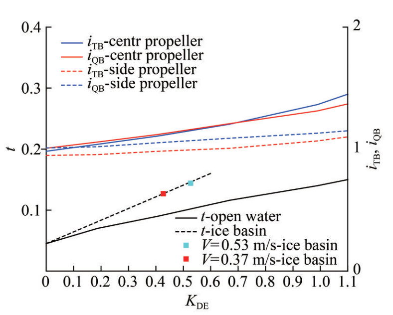Figure  11  Alternative interaction coefficients as a function of the parameter K_DE obtained in hydrodynamic and ice basins for the triple-shaft icebreaker model

Download: Full-Size Img

The analysis of the presented results leads to the following conclusions. The effect of ice cover on the coefficient of hull influence on thrust i_TB and the coefficient of hull influence on torque i_QB is relatively minor. Therefore, based on the state-of-the-art knowledge of physical processes, these coefficients are assumed not to change significantly in ice.

The thrust deduction coefficient t is notably increased. This fact should not be surprising because theoretical studies on the interaction of an ideal propeller with a solid body indicate that the thrust deduction coefficient should increase in such cases (Basin and Miniovich, 1963). These theoretical considerations only suggest the trend in the thrust deduction coefficient variation but do not allow us to calculate its value due to the use of a highly simplified propeller model and the assumption of an ideal fluid. However, the increase in the thrust deduction coefficient in ice may necessitate some adjustments in the self-propulsion test procedures in ice basins. This aspect highlights the importance of further investigation into the physical laws governing propeller/hull interaction in ice.

4   Conclusion

A novel approach for defining ship propulsion parameters in ice shows great promise. This method is based on a new alternative system of coefficients that describe propeller/hull interaction. The system is valid and effective at small advance coefficients J ≤ 0, 3, which is typical for a ship operating in ice conditions where the wake fraction w is often negative.

An important aspect of the alternative interaction coefficients is that they can be derived using traditional data from hydrodynamic and ice experiments. Essentially, these alternative interaction coefficients are obtained through minor changes in processing technologies for established experimental relations. Equally important is that the equivalence of the alternative and traditional interaction coefficient systems was demonstrated with such accuracy that no scale effect was observed (Kanevskii and Klubnichkin, 2017).

The alternative interaction coefficients enable comprehensive calculation of ship propulsion in ice during the design phase, including propeller effective thrust, number of revolutions, consumed power, and ship speed. These calculations not only allow for more accurate predictions of the ice performance of a designed ship by correcting the definition of the effective thrust but also provide inputs for ship power and automation system designers. Overall, this method can enhance the accuracy of determining propulsion power for a vessel already in the design phase. Preliminary calculations of ship propulsion and thrust characteristics in ice would allow for the prediction of full-scale ice resistance without the need to measure propeller thrust during sea trials. Measuring propeller revolutions, ship speed, and the power delivered to propellers is sufficient to determine propeller thrust. These measurements can be conducted using standard instruments on board.

The experimental methods described here enable the determination of alternative interaction coefficients not only in hydrodynamic basins but also during self-propelled model tests in ice. The ability to compare alternative interaction coefficients determined in hydrodynamic and ice basins opens the way for investigating how these coefficients are influenced by ice conditions. This analysis will allow for the exploration of interaction coefficients specific to ice conditions and their application.

Calculating ship propulsion performance in ice offers new opportunities for analyzing data obtained during full-scale ship trials in ice.