1   Introduction

In liquid flow, when the pressure drops to the saturated vapor pressure at the corresponding temperature, the liquid can form vapor-filled cavities (Hu et al., 2013). This phenomenon usually leads to damage to the engineering devices caused by collapse. People's understanding of cavitation initially originated from the cavitation phenomenon of ship propellers, which was discovered in 1895 when Barnaby and Parsons studied the severe decrease in propeller thrust at high speeds. Subsequent researchers found that cavitation is commonly present in devices containing liquids, such as water pumps and turbines. The phenomenon of cavitation is a crucial research topic and has been studied for more than 100 years. From an engineering perspective, cavitation often reduces the performance of hydraulic machinery, generates vibration and noise, and can cause severe impact erosion in materials. However, it benefits underwater vehicles in high-speed motion. Utilizing technologies and theories to improve the speed of underwater vehicles remains the focus of study for many domestic and overseas researchers (Wang et al., 2015). This research will greatly reduce the friction resistance between a vehicle and liquid when the vapor-filled cavity wraps the vehicle during movement. Thus, it will become the main method for resistance reduction of future underwater vehicles.

However, many difficult issues exist because of the cavities, which accompany many complicated physical phenomena, such as multiphase flow (Nguyen and Park, 2022), unstable phase boundaries (Yoon et al., 2021), and cavity collapsing effects (Fan et al., 2021). Supercavitating vehicle research is hard to crack because of these factors. In particular, it is difficult to establish a perfect mathematical model of vehicle motion that contains all the uncertainties. During the underwater motion of a supercavitating projectile, its navigation state completely depends on the initial conditions (Wang et al., 2020), hydrodynamic environment (Xu et al., 2023), and structural parameters (Wang et al., 2023), which directly determine whether the projectile can achieve the goal of damage. These three factors can be summarized into two categories: the influence of the dynamic parameters of the body itself and the external influence.

Recently, with the improvement of the accuracy of supercavitating projectile models, researchers (Mirzaei and Taghvaei, 2019; Daijin et al., 2020; Zou et al., 2021; Wang et al., 2023; Zou et al., 2023) have conducted a large amount of research on structural optimization design based on the established mathematical models. Accompanying this research is a dynamic analysis of the body. Rand (1997) conducted in-depth research on the flight dynamics characteristics of simplified supercavitating projectiles, focusing on the tail-slap frequency of supercavitating projectiles, assuming that the body rotates in a plane around the head. The results indicate that the tail-slap frequency increases with decreasing navigation speed, and the collision frequency depends on the initial conditions. He (2013) combined Richard's theoretical method with the finite element method to establish a bidirectional fluid–structure coupling program. He obtained not only the dynamic behavior of the body but also the tail-slap action load, and the dynamic results were consistent with Richard's results. Furthermore, Zhao et al. (2019) proposed the mirror hypothesis of tail-slap and simulated the motion of a supercavitating projectile based on Richard's theory. As the number of tail-slaps increased, the tail force gradually decreased. The instability mechanism of supercavitating vehicles was preliminarily analyzed in this work.

Although the Richard model has preliminarily revealed the motion laws of supercavitating projectiles, it is too simple to deeply reveal the stability characteristics. Kulkarni and Pratap (2000) analyzed the force characteristics of the tail-slap of a supercavitating projectile and proposed a three-degree-of-freedom model in the longitudinal plane. The mass distribution characteristics of the body were studied. The results showed that although the projectile has a tail-slap effect, the motion trajectory remains essentially linear, the frequency shows a parabolic distribution throughout the motion process, and its maximum value decreases with the moment of inertia. On this basis, Nguyen Thai et al. (2018) considered the influence of attack angle and established a more accurate three-degree-of-freedom model, which was verified through launch experiments. The model's velocity error was 1.1%, providing a theoretical basis for supercavitating projectile design.

Miezaei et al. (2015) further established a six-degree-of-freedom mathematical model for supercavitating vehicles. The model combined different planning forces, Logvinovich (Mao, 2010), Hassan (Yen et al., 2011), and empirical (Mirzaei et al., 2015), with bubble models, Zhang (Guo et al., 2012) and Vlasenko (Vlasenko, 2003), for comparison, proving that the empirical model is more accurate than existing models. Considering the applicability of the current model, Wang et al. (2020) combined the work of Mirzaei et al. (2015) and Semenenko and Naumova (2012) to further establish a dynamic model and structural optimization method for a high-speed supercavitating projectile.

In their model, the above researchers used the vertical assumption for the direction of the planning hydrodynamic force; that is, the force direction is vertical and upward with the axis of the projectile. In fact, the complexity of the fluid – structure interaction and the nonuniformity of the bubble makes it difficult to accurately predict the specific direction of the force on a supercavitating projectile during the fluid–structure interaction (Zhang et al., 2023). At the same time, because of the limitations of the current underwater measurement technology, it is difficult to completely and accurately capture the specific position of the tail-slap of a supercavitating projectile on the supercavity surface, and the randomness of the interaction between the supercavity and the body is difficult to quantify, so the theoretical research is still conducted under the premise of a hypothesis, an important factor restricting the theoretical breakthrough of the supercavitating projectile.

Thus, it is essential to establish a model that considers the randomness and instabilities of underwater environments. The main purpose of our research is to find a theoretical method for predicting these phenomena and help researchers recognize the nature of the issue clearly. Unfortunately, no such universal or commonly accepted model is available.

Some supercavitating projectile experiments demonstrate that tail-slaps occur from beginning to end for high-speed projectiles. In this paper, a normal distribution (ND) model of tail-slaps is established to describe the dynamic behavior of a supercavitating projectile underwater. The randomness and uncertainty of the underwater environment are considered by the variance of the ND. The slap effects are simulated successfully, revealing the influence factors of the number of tail-slaps. A tail-slap diagram is obtained by combining the Logvinovich expansion equation, the Gaussian distribution model, and Kulkarnis's (Kulkarni and Pratap, 2000) results. Moreover, this tail-slap diagram accords well with Richard's research. Meanwhile, the results of a single-factor ANOVA analysis of the simulation indicate that the closer the centroid is to the projectile nose, the fewer the tail-slap numbers will be. The projectile has better stability under this condition. Additionally, the initial angular velocity is larger, and the number of tail-slaps is much greater.

2   The ND model for a supercavitating projectile

2.1   Statistical law of supercavitating projectile tail-slaps

The tail-slap is a fluid – structure coupling and strongly nonlinear process, whose essence is a series of impacts between projectile and cavity. Although extensive research has been conducted on tail-slaps, studies investigating them in space are scarce because of their complexity. Moreover, the current test equipment cannot obtain the required results, such as tail-slap motion in the cavity cross section. From this aspect, the tail-slaps must be studied in space.

Most researchers believe that supercaviting projectile tail-slap motion is mainly on the top and bottom of the cavity cross-section. However, this belief is valid for supercaviting projectiles but for supercavitating projectiles. Broadly speaking, supercavitating projectiles have large mass and control systems. The tail-slap force can be weakened by controlling the posture of the supercaviting projectiles. In addition, the tail-slap motion will be restrained in the vertical direction because of the large mass. Contemporary researchers do not fully understand underwater projectile motion. However, much of the experimental data and simulation results from previous literature (Schaffar et al., 2012) suggest that the tail-slaps are not on a plane, but a random motion with some statistical law in the cavity. Figure 1 shows underwater projectile tail-slaps captured from the side of the projectile. It is obvious that the tail-slaps mainly occur on the side of the cavity rather than in a vertical plane.

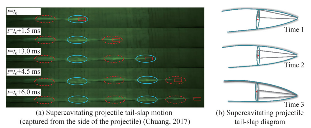Figure  1  Supercavitating projectile tail-slap

Download: Full-Size Img

Figure 2 was also captured from the side of the projectile. Obviously, the adjacent slap positions are not in a vertical plane, which is the same phenomenon experimentally observed in the paper (Chuang, 2017). This evidence proves that the supercavitating projectile slaps in the cavity are a series of space motions with strong randomness and uncertainty. For adjacent tail-slaps, the second position is not strictly rotating the first one 180° but distributes near the first one added 180°. Therefore, the adjacent tail-slap positions have the characteristic of an ND. Therefore, it is meaningful to conduct theoretical research on this phenomenon to propose a mathematical model for it.

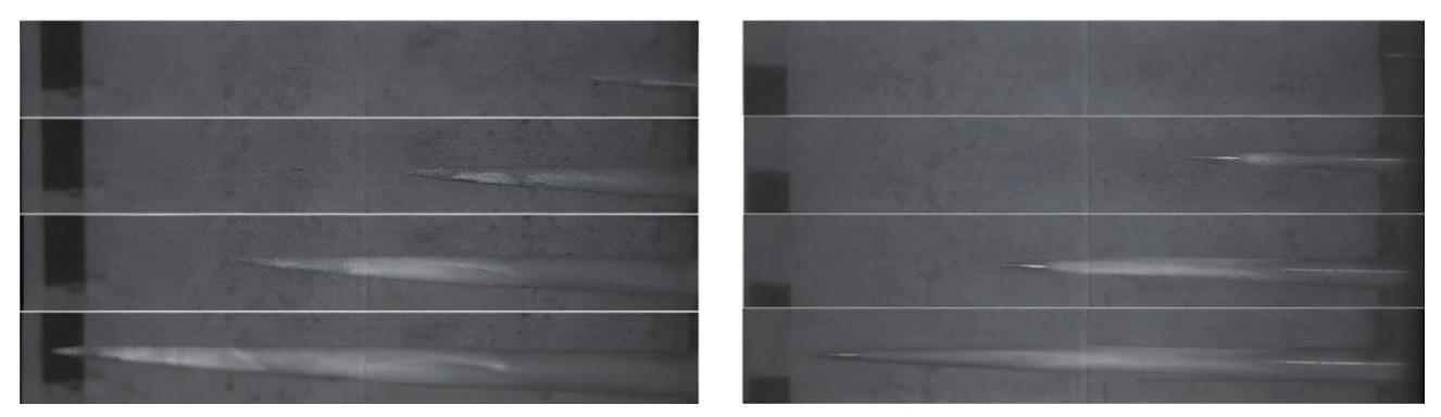Figure  2  Supercavitating projectile tail-slap motion (Li et al., 2018)

Download: Full-Size Img

According to the experimental results, the most likely latter tail-slap position is to rotate 180° at the former. However, the probability gradually decreases to 0 from the latter position to the former position along the cavity boundary, which approximately obeys an ND. Therefore, a 3σ-NDSM in the cavity can be established on the basis of the ND, as shown in Figures 3 and 4. As the ND is defined on (−∞, +∞), it must be redefined to make it physically meaningful. Thus, a 3σ- NDSM is established on a random process. In terms of universality and accuracy, the study of this model is more important than that of the two-dimensional model.

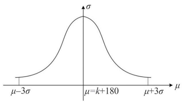Figure  3  Normal distribution model

Download: Full-Size Img

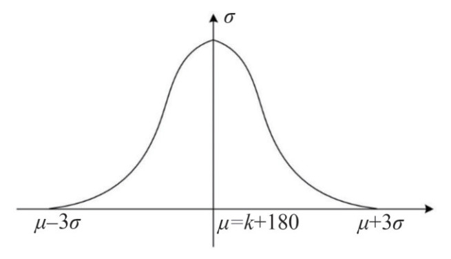Figure  4  Improved 3σ-NDSM

Download: Full-Size Img

Figure 5 is a sketch of tail-slaps, which is a cavity cross-section at the projectile's tail. The former tail-slap occurred at this moment, and thus, the latter tail-slap position depends on the direction of the exciting force. There are many models for calculating the magnitude of this force, but it is difficult to determine the direction of the force because of the complexity of fluid-structure coupling. Therefore, the 3σ-NDSM is proposed to determine the direction of the exciting force, which is based on the statistical law of the experiment.

Figure  5  Supercavity section at the tail of a projectile

Download: Full-Size Img

2.2   ND and 3σ-NDSM

The ND is the general law of many random events in nature, such as human height, weight, measurement error, and crop yield. All mentioned above have the characteristics of an ND. Therefore, the ND is widely used for practical problems and has a universal importance in nature.

Generally, the ND probability density function of random variable X is

where μ and σ > 0 are constant, and the random variable X obeys an ND. μ and σ² are ND parameters, recorded as X~ N(μ, σ²).

Because the tail-slap position distribution and the ND are very similar, it is assumed that the random variable of slap direction θ obeys an ND; that is, θ~N (μ, σ²), where μ is the mean, and σ² is the variance. The random variable θ is defined as each time tail-slap direction, which is shown in Figure 6. The probability density function of X is defined on the real field R. In fact, the tail-slap direction θ must change in the range of [0°, 360°] for a physics problem. Therefore, θ must be constrained in the interval [0, 360]. Obviously, the mathematical ND model is not suitable here. A 3σ-NDSM that matches the actual problem must be adopted.

Figure  6  Cavity cross-section scale

Download: Full-Size Img

According to the 3σ principle of an ND, if θ~N (μ, σ²), the probability of θ is 0.997 3 when we let X change in (μ−3σ, μ+3σ); otherwise, the probability is only 0.002 7; that is, θ can hardly be selected from the interval (μ−3σ, μ+3σ). In Figure 6, the cavity cross-section at the projectile tail is divided into several equal parts from 0 to 360, which are set as the 3σ intervals. The ND probability density function of X is defined on [0, 360], omitting those cases outside the interval, which is defined as 3σ -NDSM. Therefore, 3σ-NDSM has more actual meaning.

2.3   The ND assumption of tail-slaps

For convenient analysis, the following descriptions of tail-slap are made according to the experimental results: The initial slap position is difficult to determine because of the uncertainty produced by the initial factors. These factors include the disturbance of gunpowder gas during the middle trajectory, the change in the cavity layer from cloud cavity to supercavity, and so on. All the abovementioned disturbances are the reasons why the initial slap position is uncertain.

Figure 7 shows the inhomogeneity of the cavity. This figure shows that the disturbance is as complex as the flow. The disturbance for the projectile is mainly about the trajectory of the projectile motion in the cavity. According to the Euler dynamic equations, the projectile trajectory relies on the Euler angles. The Euler angles depend on the angular velocity. Since the projectile impacts the cavity continually from beginning to end, angular velocity is a vital parameter in supercaviting projectile research. Given the complexity of the initial disturbance, the initial slap position is not located in the cavity's top or bottom.

Figure  7  Disturbance of multi-factors for supercavitating projectile (Liu et al., 2015)

Download: Full-Size Img

Therefore, in the current literature, such as the nonlinear dynamic analysis of supercavitating projectiles (Lv et al., 2017), initial values usually are set as arbitrary. These initial values are selected blindly; that is, researchers select a certain range for initial parameters to calculate dynamic systems in this range. To make the results have general importance, the following assumptions are made:

1) The period from the time when the projectile exits the bore to the time when it is in free flight from gunpowder and various disturbances is called the aftereffect period of the projectile in the intermediate ballistics. In the aftereffect period, the airflow continues to accelerate the projectile and exert new interference, forming the initial disturbance of free flight and increasing the dispersion of the projectile. Aftereffect period disturbance is an important factor affecting projectile dispersion and has been introduced into the concept of initial disturbance as a research topic of exterior ballistics for many years. The lateral disturbance to the projectile has many causes, such as projectile motion in the bore and the aftereffect period.

It is proved theoretically and experimentally that the lateral disturbance is a main cause of projectile dispersion. In particular, the core of the fin-stabilized shelling penetrator is a thin rod with a large aspect ratio. When the projectile moves in the bore, various disturbance factors are more complex, including the lateral vibration caused by the projectile bore gap, the deflection caused by the longitudinal acceleration of the projectile, the lateral movement of the core clip relative to the bore wall, and the yaw of the core relative to the clip. Because of the complex stress condition, once the design is improper, the projectile body will be deformed or even fractured, severely affecting the normal flight. Particularly in an underwater environment, in addition to the disturbance of gas to the projectile, there are also many bubbles at the muzzle, and the complex fluid–solid coupling effect is generated between the bubbles and the projectile. Driven by so many complex forces, the projectile will initially be in a random distribution state, so a uniform distribution is the most convenient for describing this type of disturbance.

The initial tail-slap location obeys a uniform distribution on the cavity cross-section of the projectile tail and is influenced by fluid disturbance. That is, the initial slap position may occur anywhere in the cavity cross-section [0°, 360°], and the opportunity is equal.

2) Because water is 800 times denser than air, and the supercavitating projectile moves at a high-speed underwater, the hydrodynamic force is 100 orders of magnitude higher than the aerodynamic force. The supercavitating projectile given in the literature (Zhu and Li, 2022) is 0.056 kg, and its planning resistance can reach 550 N, which can be converted to a mass of approximately 56 kg, 1 000 times that of the supercavitating projectile. Therefore, the mass of the supercavitating projectile can be ignored in a simulation calculation.

It is assumed that the trajectory of the projectile tail at the cavity cross-section is a straight line.

3) In the interaction between a supercavitating projectile and a supercavity wall, the supercavity will generate a restoring force on the projectile, causing the projectile to produce the effect of a tail-slap. However, the author believes that there are many uncertainties in the fluid–structure interaction, which is difficult to predict completely and accurately. Therefore, the "vertical hypothesis" on the planning force cannot truly reflect the direction of force that acts on a projectile. At the same time, in many test results, the high-speed images captured are observed on a plane, which cannot truly capture the specific position of the tail of a supercavitating projectile. However, the nonplanar characteristics of the tail-slap motion can also be observed from a two-dimensional plane.

The latter tail-slap position is most likely to be rotated 180° around the former's position, which has the property of an ND. Therefore, the adjacent tail-slap positions are always correlated. Suppose the tail-slap position k obeys the ND of parameters μ and σ², which is recorded as k~ N (μ_i, σ²). When a consecutive tail-slap process is considered, μ_{i + 1} = k+180, σ = f (ρ, R), μ_{i + 1} is the angle of the expected later slap position, ρ is the curvature radius of the cavity, and R is the curvature radius of the projectile tail, where the standard deviation σ is proportional to ρ. σ is inversely proportional to R.

4) After the supercavitating projectile interacts with the supercavity, the supercavity shape will be distorted. According to Logvinovich's cavity independent expansion principle, the independent deformation of the distorted supercavity section will not transmit disturbance forward or backward. Therefore, the newly formed supercavity will remain undisturbed after the next tail-slap. This conclusion is clearly reflected in Figure 1(a).

It is assumed that the cavity deformation-caused tail-slaps are neglected. Meanwhile, the section of the projectile tail is simplified as a point during the plotting of the tail-slap image.

Figure 8 demonstrates a tail-slap diagram of a supercavitating projectile. During the tail-slaps, the cavity cross-section shrinks at the projectile tail because of the attenuation of projectile velocity. The ND law still holds on the cavity cross-section after shrinkage. The mean value μ of the ND is the former angle added with 180°. In addition, the standard deviation σ, which depends on the cavity radius at the projectile tail, needs to be recalculated each time. That is, σ needs to be updated according to the reduction of the cavity. Based on hypothesis 3), σ will be smaller after each tail-slap. The angle of the latter tail-slap is close to that of the former tail-slap but rotated by 180°. Because of the motion of the projectile, the tail-slap direction is more concentrated, and the randomness is weakened.

Figure  8  The tail-slap diagram of supercavitating projectile

Download: Full-Size Img

3   Tail-slap stochastic mathematic model and simulations

3.1   Tail-slap stochastic mathematic model

1) Initial tail-slap uniform distribution model

According to hypothesis 1), the initial tail-slap position is random, so it is considered to create a mapping between angles and real numbers from 0 to 360. The initial opportunity of the tail-slap position is equal at every position, and the uniform distribution probability density function of x is set in the range of [0, 360]. Thus, the uniform distribution probability density function is defined as follows:

where x is the image of angle θ mapped on the real number field R.

2) The 3σ-NDSM

The 3σ-NDSM can simulate the tail-slap phenomena. In this model, μ reflects an average level of the latter tail-slap position. That is, the value of μ at the current position is k+ 180. The parameters k_i and μ_i can be obtained using the following procedure.

The first step: k₁~U (0, 360)

The second step: μ₂ = k₁+180, k₂~N (μ₂, σ²)

The third step: μ₃ = k₂+180, k₃~N (μ₃, σ²)

…

The formula of the algorithm is μ_i+1 = k_i+180, k_i+1~N (μ_i+1, σ²)

σ reflects the deviation of the latter tail-slap from μ. To determine the parameter σ, much experimental statistical data is required. This requirement is unrealistic, so this paper proposes two methods for determining σ from estimation and analysis.

a. Approximate solutions of σ

For 3σ-NDSM, the integral value of the probability density function is greater than 0.997 3 in the interval [k, k+ 360] according to the 3σ principle of the ND. Its expression is as follows:

For Equation (3), let t = (x−μ)/σ:

Letting m = 2^0.5t/2, Equation (4) can be written as

As μ is in the interval [k, k+360], the inequality k < μ < k+360 is established and μ satisfies:

That is

Therefore, the inequality in Equation (5) can be expressed as

According to the property of integral, Equation (5) can be rewritten as follows:

Generally, the Gauss error function with variable m can be defined as

The term on the left side of Equation (9) is replaced by Equation (11), which is obtained from the properties of the Gauss error function.

Equation (7) is substituted into Equation (11):

Since the Gauss error function is an odd function, Equation (12) can be arranged as follows:

By consulting the Gauss error function table, we see that

If linear interpolation is applied to Equation (14), we obtain:

Because the Gauss error function is monotonically increasing on [0, +∞], the following inequality holds:

σ is the standard deviation of the ND and σ > 0. The range of the standard deviation in a mathematical sense can be obtained as follows:

Finally, a 3σ-NDSM is established.

b. Analytical formula of σ

It is considered that the variable x of the ND probability density function is limited to the interval (−∞, +∞) to [k, k+ 360]; then, Equation (3) can be written as

For Equation (19), let t=(x−μ)/σ:

Letting a = t−(k−μ)/σ, Equation (20) be written as

By simplifying Equation (21), we obtain:

The left-hand side of Equation (22) is expanded using a power series. It is expressed as

Equation (7) is substituted into Equation (23):

In theory, the value of σ can be obtained by solving Equation (24) for σ, which is difficult to do, so the estimation interval value of σ in a can be used to solve for σ.

c. σ −κ estimation equation

To obtain σ conveniently, a σ estimation equation is proposed based on the σ approximate solution and the experimental phenomenon that adjacent tail-slap positions are always nearly symmetric about a cavity diameter. Dimensionless κ is defined according to hypothesis (3):

where δ is the supercavity radius at the body's tail, and R is the radius of the projectile's tail. When the cavity crosssection at the projectile tail is equal to the projectile tail crosssection, the value of κ is set as 1. At this moment, the projectile tail-slaps will not occur, which is equivalent to the ND with zero standard deviation. Therefore, σ and κ have a functional relation. The maximum cavity cross-section at the projectile tail corresponds to the maximum kinetic energy of the projectile. Currently, the value of the σ is 59.84 and κ is κ₀. There are two groups of data, which are composed of κ and σ, (1, 0), (κ₀, 59.84). Suppose the equation of σ−κ can be obtained using a linear relationship because σ and κ are positively correlated:

where κ is the updated value at each tail-slap, and κ₀ is the value of the initial tail-slap.

3) Logvinovich independent expansion model of cavity

Suppose the fluid is incompressible potential flow, the linear motion of the projectile underwater is considered, and the projectile moves at an initial velocity v₀ and attenuates according to the law of inverse proportional function (Wang et al., 2019). The velocity expression is as follows:

where m is the mass of the projectile, ρ is the fluid density, A is the section area of the cavitator, C_x0 is the drag coefficient, which is set as 0.82, and t is the flight time of the projectile.

The saturated vapor pressure inside the cavity is p_v, the ambient pressure is p, and the cavity cross-section is S. Logvinovich derived the independent expansion equation of the cavity based on the potential flow theory according to the energy conservation equation (Wang et al., 2019).

where the coefficient k′ weakly depends on the number of cavitations σ = Δp/(0.5ρv²). Generally, k′ = 4π/(A²) and A ≈ 2 is an empirical constant, x′ is a certain cavity crosssection along the cavity length, and l is the cavity length.

To simulate tail-slaps, the cavity cross-section of the projectile tail must be calculated. When a cavitator moves through a region of space, the cavity expansion time is equal to the time that the projectile moves a length of L. Therefore, there is

where t_k is the expansion time of the cavity at a certain position, that is, the time in which the projectile moves a length of L, and L is the length of the projectile.

By integrating Equation (29), t_k can be obtained (Wang et al., 2019):

3.2   Simulation method for supercavitating projectile tail-slaps

1) Initial conditions

a. The initial velocity of the supercavitating projectile is 300 m/s when it is launched underwater;

b. The mass m of the supercavitating projectile is 0.1 kg;

c. The length L of the supercavitating projectile is 156.81 mm;

d. The fluid medium is water with a density of 1 000 kg/m³;

e. The maximum diameter D of the supercavitating projectile is 12.67 mm;

f. The diameter of the projectile cavitator is 4.49 mm;

g. The gravitational acceleration g is 9.8 m/s²;

h. The atmospheric pressure P₀ is 101 325 Pa;

i. The projectile motion depth h is 2.3 m;

j. The saturated vapor pressure P_v is 3 025 Pa at 24 ℃;

k. The rotational inertia of the projectile around the center of mass on the plane is 1.46×10⁻⁴ N/m;

l. The distance x_cm between the center of mass and the projectile tail is 80 mm;

m. The time step t is 10⁻⁵ s;

n. The total calculation time is 0.5 s.

2) Determination of the initial tail-slap position According to the experiments and analysis in Section 1, the initial position can be influenced by many factors, and the uncertainties are often complicated. During the initial tail-slap, the cavity at the projectile tail transfers from a cloudy or stratified cavity to a supercavity, and the integral cavity surface will form gradually. The initial slap position may occur in any position of cavity. Therefore, the initial position can be selected using the generated random numbers on [0, 360], which obey a uniform distribution.

3) Calculation of the cavity cross-section at the projectile tail position

Since the pressure used in Logvinovich's bubble expansion equation is not near the bubble pressure but infinite, we have p = p₀ + ρgh;

Supposing that τ is the formation time of section x, the integral of the Logvinovich bubble expansion equation can be obtained:

Let t_m = t, n ≤ i ≤ m, discretize Equation (31) using the complex Simpson formula, and let f = (t − u) (p − p_v):

The formula for calculating the cavity section area of the projectile tail can be obtained by substituting Equation (30) into Equation (32):

4) Calculation of the tail-slap positions

The initial tail-slap position is determined using the uniform distribution. This information is used to calculate the next tail-slap expectation μ_{i + 1}, μ_{i + 1} = k_i+180 (i = 1, 2, 3, …, n); then, σ is determined using Equation (26), where k_i is the angular value of the current tail-slap position.

The value range of k_i and μ_i+1 is [0, 360]. When 180 is added to k_i, the result might exceed the range of [0, 360], and it has lost physical meaning. Therefore, every μ_i+1 must be limited and then recorded as μ_i^*. The limited calculation method is as follows:

where n is a left integer function expressed as follows:

Meanwhile, a negative mathematical expectation may also occur when calculating the next time step. Applying the geometry method to the cavity cross-section at the projectile tail position, the negative angle can be defined as positive from 0° to 360° so that the calculation results have physical meaning. Based on the above, an algorithm is performed as follows:

Step 1: When |μ_{i + 1}| > 360 go to step 2, else go to step 7;

Step 2: n = [|μ_{i + 1}|];

Step 3: ξ_i = |μ_{i + 1}|−360n;

Step 4: μ_{i + 1} = ξ_i sign(μ_{i + 1});

Step 5: If sign(μ_{i + 1}) = −1 is true μ_{i + 1} = 360−ξ_i, else go to step 6;

Step 6: μ_{i + 1} = ξ_i;

Step 7: If sign(μ_{i + 1}) = −1 is true μ_{i + 1} = 360+ξ_i, else go to step 8;

Step 8: μ_{i + 1} = μ_{i + 1}.

The polar coordinate system is established by setting the origin at the center of the cavity cross-section at the projectile tail, in which the polar center is O and the axis is r, and the position of each tail-slap can be determined by k_i:

where k_i is the last tail-slap position based on polar coordinates. The unit "degree" in the original image is used to calculate k_i, in which only the unit needs to be changed and the value need not be changed. x_i and y_i are the current tail-slap coordinates in a polar coordinate system.

5) Determination of the relation between adjacent tail-slaps

The supercavitating projectile experiences two stages in the process of underwater motion, which are the motion completely inside the supercavity and the motion interaction between the projectile and the supercavity. Consequently, the angular velocity curve of the tail-slap of the supercavitating projectile is oscillatory. To explain this variation, a map that relates the angular velocity before impact to the angular velocity after impact is established by Kulkarni (Kulkarni and Pratap, 2000). Figure 9 shows the results of a tail-slap.

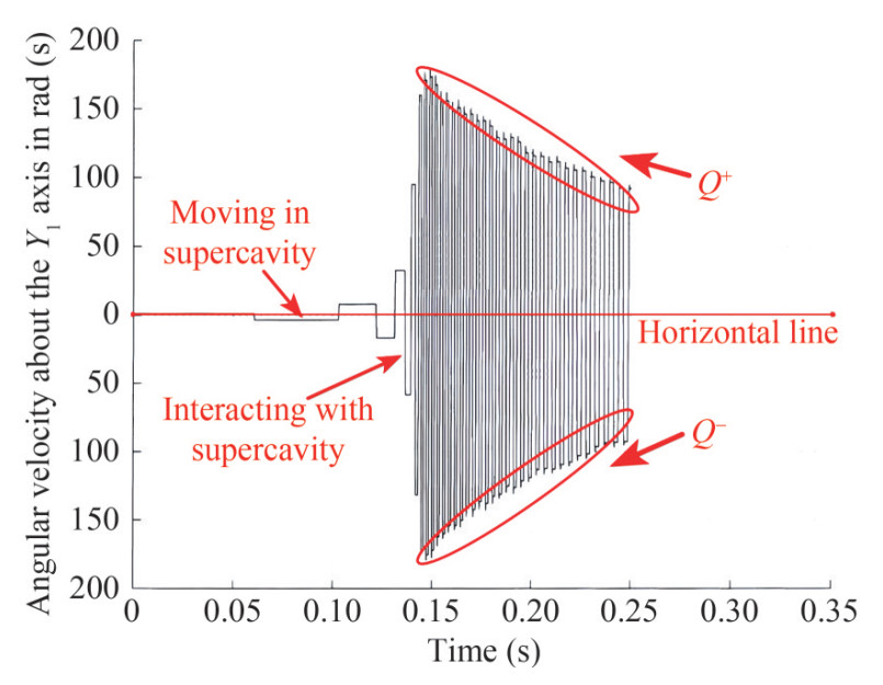Figure  9  Tail-slap process of a supercavitating projectile (Kulkarni and Pratap, 2000)

Download: Full-Size Img

Kulkarni and Pratap (2000) established the 3-DOF tailslap equation of a supercavitating projectile in a plane, which calculated the tail-slap angular velocity curve of two types of projectiles. On the basis of the dynamic analysis results, Kulkarni derived the angular velocity formula before and after the tail-slaps:

This equation has considered all the dynamic factors, including projectile parameters and exciting force, so there is no need to present the exciting force formula. The detailed work is in the literature (Kulkarni and Pratap, 2000):

Q⁻ and Q⁺ are the angular velocity of the supercavitating projectile before and after a tail-slap, respectively. e is the compensation coefficient, and its expression is

where U⁻ is the velocity of a supercavitating projectile, and α is the pitch angle, that is, the angle between the projectile axis and the wall of the cavity when the projectile tail-slaps. α can be expressed as

If the coordinates of the first and second tail-slaps are (x₁, y₁) and (x₂, y₂), respectively, the plane distance between the two positions is

The linear velocity at the projectile tail is

Thus, the time interval between two tail-slaps is obtained as follows:

Salil S. Kulkarni's results (Kulkarni and Pratap, 2000) are proposed on a plane. According to hypothesis 2), a supercavitating projectile has a linear tail trajectory, so a plane is approximately formed between two tail-slap positions. It is effective to apply Salil S. Kulkarni's conclusion (Kulkarni and Pratap, 2000) between two tail-slaps.

6) Determination of the initial slap angular velocity

The initial tail-slap angular velocity is disturbed by many uncertainties, so it can be set arbitrarily. When the actual tail-slaps are simulated, the initial angular velocity of the tail-slap can be selected as any number. When the influence of some parameters is studied during the projectile motion, the same initial slap angular velocity of the projectile can be used.

7) Computing termination condition

When the cavity cross-section of the projectile tail is less than or equal to the projectile tail cross-section, the cavity collapses completely, and the tail-slap phenomena disappear. The theory in this paper is no longer applied. Therefore, when Equation (44) is satisfied, the calculation will terminate.

4   Analysis of the simulation results

The tail-slap simulation method proposed in this paper can predict and simulate the tail motion of a supercavitating projectile. Because this model is based on probability theory, the results of each calculation are different. Therefore, much data must be employed for statistical analysis.

4.1   Tail-slap difference at the same initial angular velocity

To study the tail-slap difference of projectiles at the same initial velocity, the initial angular velocity Q⁻ is set as 2 rad/s, the flight distance x is set to 20 m, and the centroid x_cm is set as 80. Based on the tail-slap model proposed above, Figures 10, 11, and 12 are the diagrams of tail-slaps under an initial velocity of 300 m/s, in which the number of tail-slaps in cases 1, 2, and 3 is 20, 3, and 15, respectively. The x and y axes represent the magnitude of the cavity cross-section on the plane. The different colors of the circle are the cavity cross-section outline at different times. The mark of the start is the projectile tail position.

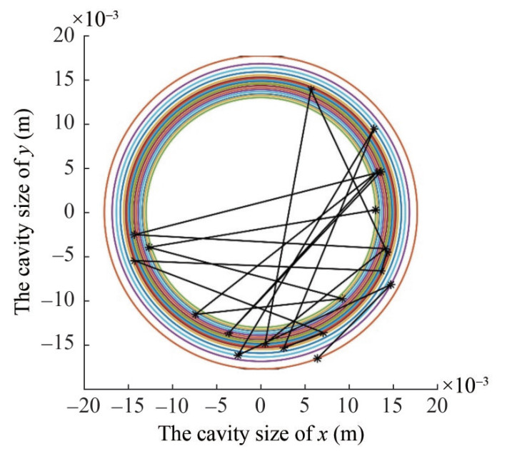Figure  10  Tail-slap case 1 at an initial velocity of 300 m/s

Download: Full-Size Img

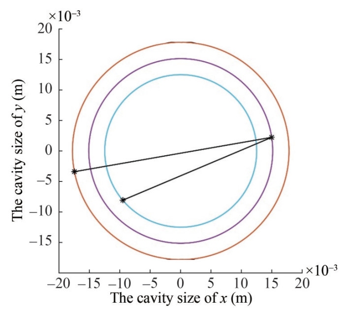Figure  11  Tail-slap case 2 at an initial velocity of 300 m/s

Download: Full-Size Img

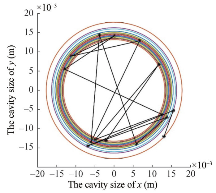Figure  12  Tail-slap case 3 at an initial velocity of 300 m/s

Download: Full-Size Img

These data indicate that under the same initial conditions, the tail-slap cases are inconsistent, which shows that the same initial conditions have different results for a certain projectile. Comparing the distance between the beginning two tail-slap positions in Figures 10, 11, and 12, we find that the distances of case 1 and case 3 are much smaller than that of case 2. Therefore, the tail-slap time interval will initially be longer for case 2, and the projectile will fly farther, which could give the cavity enough time to reduce. From the σ−κ equation, we see that the standard deviation σ decreases with the dimensionless κ. From a physical view, σ will decrease along with the cavity radius. Meanwhile, the possibility of the adjacent tail-slap distance increasing will grow continuously. In general, the number and frequency of tail-slaps will be reduced when the supercavitating projectile flies a certain distance. This result is undoubtedly beneficial to the stability of supercavitating projectiles. Therefore, it can be concluded that the tail-slap frequency of supercavitating projectiles is greatly influenced by the distance between the beginning two tail-slaps. The distance of the initial several tail-slaps determines the tail-slap frequency of the later period. When this distance is large, the tail-slap frequency will largely reduce, and vice versa. In 1997, Rand et al. (1997) proposed successive impacts from a sample simulation (Figure 13), which was based on oscillation theory. This theory makes significant simplifications about supercavitating projectiles, but we put a three-degree-of-freedom dynamic equation into this simulation. The simulation results are very similar to Richard's (Rand et al., 1997).

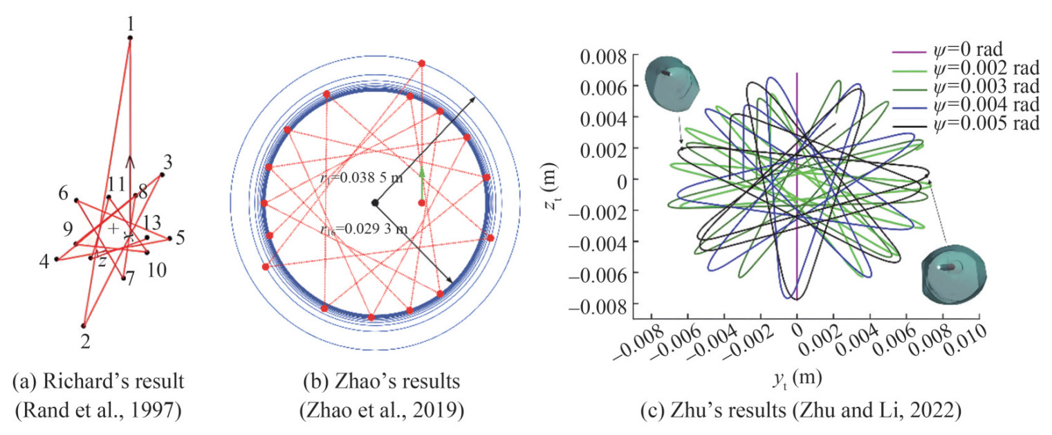Figure  13  The tail-slap

Download: Full-Size Img

Remark: In this study, the σ -NDSM tail-slap dynamic model is proposed, so every simulation result is random, and the results given in the literature are obtained under the assumption. The randomness of the model theoretically includes all the results in the literature, including the mirror reflection model of Zhao et al. (2019) and Zhu and Li (2022) results obtained by CFD. In essence, the model is more universal. Therefore, the author believes that the results of stochastic dynamics simulations are similar and not completely consistent with those in the literature.

Figures 14 and 15 show the tendency of κ and σ, respectively. To present the data tendency, a curve fit is used to fit these data. The equation of σ − κ indicates that σ is proportional to κ, so the tendency of the κ − t curve is consistent with σ − t, which shows a monotonically decreasing trend. However, the meanings differ. The κ − t curve shows that with the motion of a supercavitating projectile, the cavity radius cross-section at the projectile tail decreases gradually. The variation tendency does not change with tail-slap conditions. The σ − t curve shows that with the movement of the supercavitating projectile, the dispersion of the tail-slap decreases gradually, and the possibility of the distance between adjacent tail-slaps increasing becomes larger. Figure 16 shows the expectation curve of the tail-slaps. The expectations reflect the dispersion of the tail-slaps from the side by the fitting curves. At the beginning of the tail-slaps, the fluctuation of the expectation curve is smoother. This fluctuation increases with time. This behavior shows that the possibility of tail-slap positions being far from the expectation is greater in the early tail-slap stage, which is caused by the larger σ. At the later stage of the tail-slaps, with the decrease in σ, the dispersion of the tail-slaps greatly decreases and the expectation difference between before and after a slap becomes quite large. The maximum and minimum limitations of the expectation gap are calculated to be 180 and 0, respectively.

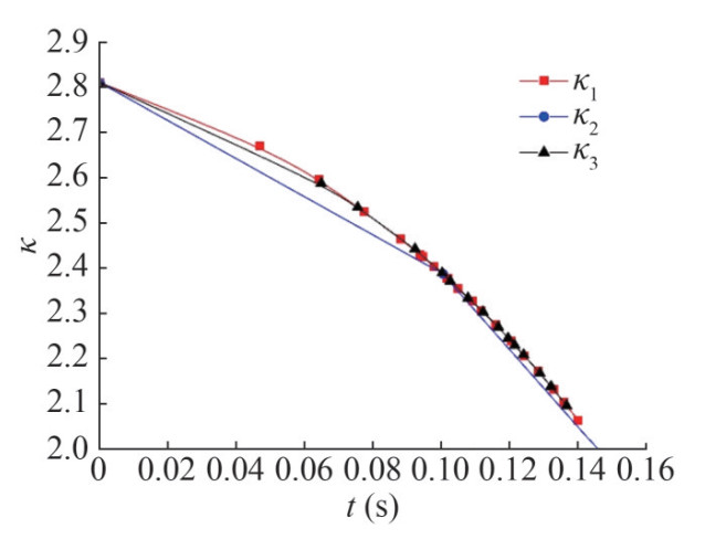Figure  14  κ variation curve in the three tail-slap cases

Download: Full-Size Img

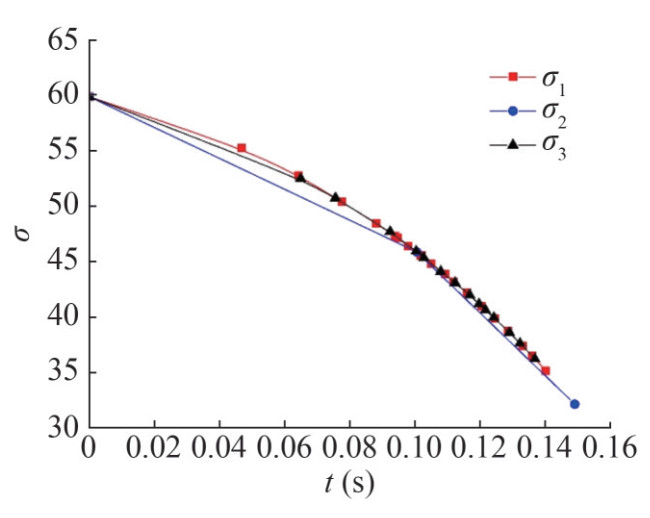Figure  15  σ curves in the three tail-slap cases

Download: Full-Size Img

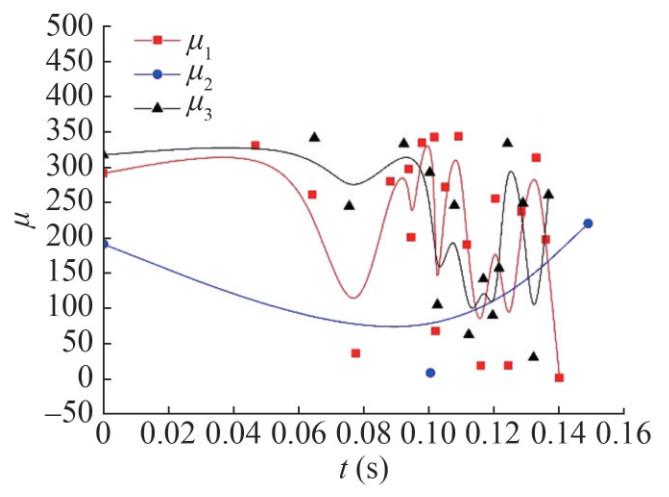Figure  16  μ curves in the three tail-slap cases

Download: Full-Size Img

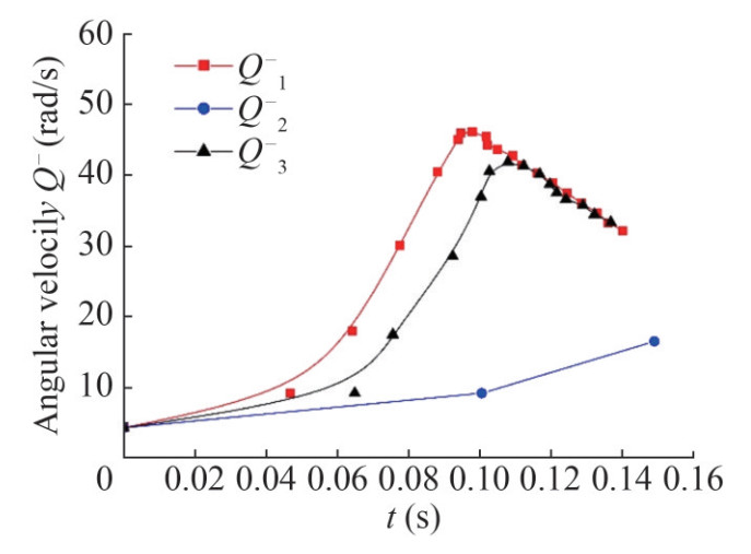Figure  17  Q⁻ curve of the angular velocity of the three tail-slap cases

Download: Full-Size Img

Q₁⁻, Q₂⁻, and Q₃⁻ given in Figure 16 are the angular velocity curves corresponding to the three cases in Figures 10, 11, and 12, respectively. The number of tail-slaps in Figures 10, 11, and 12 is 20, 3, and 15, respectively.

For supercavitating projectiles with more tail-slaps, i.e., Q₁⁻ and Q₃⁻ curves, because the planning force consumes projectile energy in the motion, it affects the range of supercavitating projectiles. The Q₁⁻ and Q₃⁻ curves showed a trend of first rising and then falling. In the rising stage, the body stability gradually weakened with the continuous tail-slapping, the energy consumption increased, the kinetic energy of the projectile decreased, and the supercavity section at the projectile tail gradually decreased. When the angular velocity exceeds the peak value, there is a sharp downward trend. At the same time, the number of tail-slaps increases sharply in a short time, indicating that the small attitude change produces a tail-slap that is caused by the supercavity section reduction. Moreover, the stability of the projectile drops sharply, and finally, the projectile loses stability. Therefore, the relationship between angular velocity and the number of slaps is mutually reinforcing, so the extremum of the case 3 curve lags that of the case 2 curve.

The peak value and the number of tail-slaps are much smaller for the Q₂⁻ curve than for the Q₁⁻ and Q₃⁻ curves, which shows that the supercavitating projectile moves smoothly. Because the number of tail-slaps is smaller, the supercavitating projectile can maintain its stability better, with a low energy decay rate and large range. The above discussion shows that for supercavitating projectiles under the same conditions, the uncertainty of the hydrodynamic direction of the tail-slap will make the same structure projectiles show different dynamic characteristics, which is also a phenomenon found by the author in many underwater projectile tests.

4.2   The ANOVA analysis of the initial difference angular velocities

Because the tail-slaps have great randomness, statistical analysis is necessary to study the motion. However, some projectile parameters cannot be obtained because of imperfect test equipment, which makes statistical analysis difficult. At the same time, statistical analysis needs a large amount of test data as a basis, which is unrealistic for expensive supercavitating projectile tests. Therefore, it is necessary to propose a numerical model from the theoretical analysis to simulate the tail-slaps of supercavitating projectiles and then conduct statistical analysis.

Table 1 presents the simulation results under the condition that flight distance x is 20 m, initial velocity v₀ is 300 m/s, and centroid x_cm is 80 mm. Suppose the sequence of random variables of the tail-slap number under different angular velocities is recorded as ξ_i (i = 1, …, 5), and meanwhile, it is a normal population with the same independent variance. There is test event H₀: For random variable sequence ξ_i (i = 1, …, 5), the expectation is consistency. The mean and variance of sample i of five populations can be calculated using Equations (45) and (46) (the results are listed in Table 2):

The mean and variance of all subsamples can be calculated from Equations (47) and (48) as 11.36 and 50.35, respectively.

where Q_e is intragroup deviation, reflecting the fluctuation degree in r groups, and u₁ is intergroup deviation, reflecting the difference degree of ε_i. Their expressions are as follows:

The intragroup deviation Q_e and intergroup deviation u₁ were 2 763.1 and 2 271.9, respectively.

According to Cochran's decomposition theorem, when event H₀ holds, Equation (52) can be used in the test statistic of H₀:

Testing the observed values of statistics:

Here, α = 0.05. Then:

Because the observation value is much larger than the look-up table value, with a confidence level of 95%, event H₀ is negated; that is, the expectation of random variable ξ_i (i = 1, …, 5) is inconsistent. Thus, it is reasonable to believe that the initial angular velocity of the tail-slap is proportional to the number of tail-slaps.

Proofof this conclusion:

Assume that the supercavity cross-sectional area at adjacent tail-slap positions are S_i and S_{i + 1}. Substituting Equation (36) into Equation (43), we obtain Equation (55):

Omitting the parentheses for simplicity, this equation can be rewritten:

If the tail-slap frequency of a supercavitating projectile is high, then a short time interval between each impact makes the supercavity cross section slightly vary, so further simplifications can be made:

For an ideal condition, the adjacent impact expectation can be expressed as

Therefore, Equation (59) can be simplified as follows:

Obviously, when increasing Q⁻ decreases the tail-slap interval, the number of tail-slaps will increase.

4.3   ANOVA analysis of the different centroids

Several constant values must be set. The flight distance x is 20 m, the initial velocity v₀ is 300 m/s, and the tail angular velocity Q⁻ is 4 rad/s. Each supercavitating projectile with a different centroid is tested 20 times. The results are presented in Table 3. They mark ξ_i (i = 1, …, 5) as the sequence of random variables of the tail-slap numbers at different angular velocities, and they are the normal population with the same independent variance. There is testing event H₁: For the random variable sequence ψ_i (i = 1, …, 5), the expectation is consistency. The observed values of the test statistics are obtained as follows using the method of ANOVA:

Therefore, with a confidence level of 95%, event H₁ is negated; that is, random variable ψ_i (i = 1, …, 5) is inconsistent. It is reasonable to believe that the centroids will affect the tail-slap phenomena. It can be inferred that the tail-slap effect will be weakened as the centroids move forward, which benefits the stability of the supercavitating projectiles. In terms of penetration, the closer the centroid of the bullet is to the head, the better the penetration effect is. This conclusion is of great importance for guiding the design of supercavitating projectiles.

Proofof this conclusion:

For Equation (60), we expand e with a Taylor series:

The variables of Equation (62) have the following orders of magnitude:

We obtain:

Thus, Equation (62) can be simplified as follows:

Substituting Equation (65) and Equation (38) into Equation (60), we obtain:

Analysis using the order of magnitude gives:

Equation (67) can be collected as follows:

When the denominator is zero, the function has a singular point, which can be expressed as

In this study, the value of x_cm is 0.308 9 and 0.004 7, respectively. The function can be defined, and the minimum value can be solved as follows:

where A is the minimum coordinates. In this study, A is (0.038 2, 0.076 4). In general, the center of mass of a projectile is designed to be located at half the body length or closer to the head. Therefore, the center of mass range is selected as [0.038 2, 0.156]. This interval is greater than the minimum value of 0.038 2. The function h (x_cm) is monotonically increasing. Thus, we can obtain the equation:

Therefore:

For the high-frequency tail-slap state, the adjacent tail-slap time t_d is smaller, and x_cm is smaller by equation analysis, which indicates that the position of the projectile's center of mass is close to the fin, proving the statistical conclusion of the ANOVA method, and vice versa.

5   Conclusions

The purpose of the current study is to determine a supercavitating projectile tail-slap model. The most obvious contribution from this study is that a 3σ -NDSM is established. Overall, this study used the idea that the tail-slaps are random, which obeys a ND. This project is a comprehensive, statistically significant investigation of a tail-slap model on a plane. The following conclusions are drawn:

1) Through many experimental observations, it is found that the same supercavitating projectile has the problem of partial projectile instability. A random tail-slap model is proposed in this paper. Using 3σ theory, the direction force of the tail-slap is introduced into the interior of the supercavity as a normal distribution, and the integral inequality and probability distribution equation are used to establish the 3σ-NDSM model. A series equation for the variance of the ND is given by the series expansion method. To solve the problem easily, the linear approximation method is used to discretize the variance, and the tail-slap process of the supercavitation projectile is simulated and analyzed by combining the supercavity equation and the simplified expressions of dynamics.

2) The tail-slap motion characteristics under identical initial conditions are numerically simulated on the basis of the 3σ-NDSM. It has been shown that the tail-slap features differ remarkably. In addition, these features are greatly influenced by the distance between the initial several tail-slap positions, which determines the projectile's later motion. When the time interval between the initial few tail-slaps is large, the supercavitating projectile can move more steadily. The projectile spends a long time inside the supercavity and has a long range with low drag compared to the projectile with more tail-slaps. For a low tail-slap projectile, the section of the supercavity at the projectile tail shrinks greatly compared to a projectile with more tail-slaps within an adjacent tail-slap time interval. Therefore, the total number of tail-slaps is smaller.

3) The model was analyzed using stochastic dynamics simulations, and the study found that the larger the angular velocity of the initial tail-slap is, the larger the number of tail-slaps. Meanwhile, the closer the projectile mass center is to the projectile head, the smaller the tail-slap number. These conclusions are validated using the ANOVA method, which has high reliability. Synchrony verified the accuracy of the statistical analysis using theoretical analysis methods. This model provides a new perspective for studying the tail-slaps of supercavitating projectiles and a new means for analyzing the stability of supercavitating projectiles.