1   Introduction

In many military applications, underwater vehicles are considered superior to surface ships for several reasons. First, the underwater detection capabilities of surface ships are generally more limited compared to those of underwater ships. Additionally, long-range weapons and satellite detection systems are less effective against submarines. Furthermore, underwater crafts offer greater combat effectiveness and flexibility due to their enhanced stealth features. These advantages have motivated countries to invest in underwater technologies for decades. Recently, in addition to traditional underwater vehicles such as submarines and surface ships such as frigates and assault boats, governments have begun incorporating versatile semisubmersible ships into their naval fleets.

Today, submersible crafts serve various purposes, including oceanographic research, tourism, and military operations. Semisubmersible naval ships are a specialized type of combat vessel with several military applications, such as information gathering, counterterrorism, fast seal delivery, and asymmetric warfare. Their most distinct feature lies in their capability to operate at-surface and underwater, leveraging the advantageous characteristics of highspeed surface crafts and submarines. At the surface, they offer high speed and maneuverability while providing stealth characteristics during underwater operations. Karabulut et al. (2024) outlined the general design features of this ship type.

Semisubmersible naval crafts feature high-speed planing hull forms. Thus, understanding the hydrodynamics of planing hulls is crucial in their design. Planing hulls have various applications at sea, particularly when speed is a priority (Savitsky, 1985). These hulls generally exhibit V-bottom shapes and transom sterns, which enhance hydrodynamic lift. This design allows boats to operate with positive trim angles and reduces the wetted length, consequently decreasing the wave resistance of the hull (Savitsky and Core, 1980). Numerous researchers have been investigating the hydrodynamics of high-speed planing hulls since the 1950s (Tavakoli et al., 2024). One of the earliest studies was conducted by Davidson and Suarez (1949), who performed towing tank experiments using Series 50 hull forms, analyzing the performance of 20 different hull form configurations. Another early experimental analysis was conducted by Clement and Blount (1963) using Series 62 hulls. Fridsma (1969) investigated the calm and rough water hydrodynamics of prismatic planing boats, testing each model in smooth water and regular waves. More recently, Najafi et al. (2020) conducted experiments on a single-stepped version of Fridsma's series, while Vitiello et al. (2022) explored the hydrodynamics of stepped planing hulls experimentally. The most widely recognized empirical model for the hydrodynamics of planing crafts was developed by Savitsky (1964), building on earlier experimental studies.

With the developments in numerical methods and computer technology, computational fluid dynamics (CFD) has gained considerable attention from researchers. Today, computational hydrodynamics plays a crucial role in ship design (Barsoum, 2000). Caponnetto et al. (2003) used Comet, a CFD-solver, to simulate the motions of planing boats in waves. Sukas et al. (2017) conducted CFD analyses using Fridsma's (1969) hull form with Star CCM+, concluding that CFD methods can successfully predict the motion and resistance of high-speed planing crafts. Hosseini et al. (2021) performed CFD simulations employing various numerical techniques on a hard-chine planing craft, while Jin et al. (2023) investigated the performance of Fridsma's (1969) hull form in calm water and rough sea conditions.

Another key aspect of the hydrodynamic design of semisubmersible naval crafts is their hydrodynamics and maneuvering during underwater operations. Research into the hydrodynamics and maneuvering characteristics of underwater vehicles has been ongoing since the 1960s. The first successful model for maneuvering underwater crafts was developed by Gertler and Hagen (1967), with subsequent improvements made by Smith et al. (1978) and Feldman (1979). Traditionally, the hydrodynamic design of submarines focused on deep water conditions (Van Terwisga and Hooft, 1988; Moonesun et al., 2017). With advancements in computational and experimental tools, more recent studies have also considered near- or at-surface operations (Amiri et al., 2018 and 2019; Dawson, 2014; Dong et al., 2022; Toxopeus, 2008; Toxopeus et al., 2012; Vaz et al., 2010). However, these studies mainly focused on conventional submarines. Hull forms of the semi-submersible naval ships differ from the conventional submarines. Conventional submarine hulls typically feature axially symmetric outer hull geometry. Conversely, semisubmersible naval ships are designed with planing hull forms to achieve high speeds at the surface and perform only shallow dives. Therefore, the hydrodynamic design of semisubmersibles should include high-speed surface conditions and near-surface shallow dive conditions.

Previously, semisubmersible naval ships have been converted from traditional fast-speed planing crafts, often with limited attention given to their underwater performance. However, the hydrodynamic design of a semisubmersible naval ship should also consider underwater operations (Karabulut, 2024). In this research, a new hull form was developed for a 15 m long semisubmersible naval ship, designed to carry nine soldiers and optimized for performance in at-surface and submerged conditions.

Designing the propulsion system of a semisubmersible naval ship requires a detailed analysis of the hydrodynamics of the hull for at-surface and submerged conditions. The overall propulsion system, including the main propulsions, engines, electric motors, and batteries, can cover 40% of the vessel's weight due to the multipurpose characteristic of the ship. In addition, the locations and sizes of the rudders should be determined based on the hydrodynamic forces acting on the hull. Thus, this study mainly aims to present an effective numerical methodology to analyze the hydrodynamic performance of a semisubmersible naval ship.

In this study, unsteady Reynolds-averaged Navier–Stokes equations (URANSE) were used in CFD analyses conducted with Star CCM+ version 2302 to assess the hydrodynamic performance of a semisubmersible naval ship. The objective is to provide detailed insights into the hydrodynamic features of these ships. The numerical analyses encompass computations of resistance, powering, trim, sinkage, and wave elevations for various speeds during surface operations, as well as hydrodynamic forces and moments under shallowly submerged conditions.

2   Methods

2.1   Geometry and coordinate system

The geometry of the hull form is presented in Figure 1. All CFD analyses were conducted at full scale using this hull form. The general characteristics of the hull are sum-marized in Table 1, where the longitudinal center of gravity (LCG) is measured from the aft perpendicular.

Figure  1  Geometry of the semisubmersible naval ship

Download: Full-Size Img

In this study, all results are presented using a right-hand coordinate system, as shown in Figure 2. The origin of the coordinate system is positioned at the center of mass of the ship, with x, y, and z axes directed forward, portside, and vertically upward, respectively. Herein, X denotes the hydro-dynamic drag force, Z denotes the hydrodynamic lift force, and M denotes the pitching moment. These forces and moments are made nondimensional using Equations 1 and 2, where ρ is the density, L is the overall length, and V is the velocity of the ship.

Figure  2  Coordinate system

Download: Full-Size Img

2.2   Mathematical formulation

The governing equations for the flow around the ship include the continuity equation and the unsteady Reynoldsaveraged Navier–Stokes (URANS) equations (Wilcox, 2006). These equations are typically expressed in vector notation as follows:

where u_i is the mean fluid velocity, and u'_i is the fluctuating component of the velocity. p, μ, and ρ u'_iu'_j represent mean pressure, dynamic viscosity, and Reynolds stress tensor, respectively.

The URANS equations remain unclosed due to the existence of Reynolds stresses. The ITTC (2011) recommends using two-equation turbulence models for accurately modeling flow around ships. Thus, the shear stress transport SST k−ω turbulence model (Menter, 1994) is chosen to model the Reynolds stresses. The SST k−ω model is an eddy-viscosity model where the kinematic eddy-viscosity (υ_T) is calculated using the following:

where k and w denote turbulence kinetic energy and specific dissipation rate, respectively, which are calculated from the following transport equations (Menter, 1994):

Auxiliary relations and closure coefficients for the SST k−ω model can be found in Menter (1994).

The analyses also involve modeling the wave field around the vessel. To achieve this, the volume-of-fluid (VOF) method developed by Hirt and Nichols (1981) is employed, utilizing the high-resolution interface-capturing (HRIC) scheme (CD-ADAPCO, 2011) to resolve the interface between water and air at each time step. In the VOF method, a volume fraction function (αi) is defined for each cell in the computational domain such that:

where α_i is the volume fraction of ith phase in a cell, V_i is the volume of ith fluid in the same cell, and V is the total volume of the cell. The transport equation for α_i is given by

where

Finally, the fluid properties, including density and viscosity, in each cell are calculated using the volume fraction average of each phase within that cell.

The coupling of the pressure and velocity fields is achieved using the semi-implicit method for pressure linked equations (also known as SIMPLE) (Patankar and Spalding, 1972). A second-order implicit method is employed for temporal discretization. The cell center-based finite volume method is used to discretize the continuity, momentum, and turbulence equations. All simulations were conducted using Star CCM+ software.

Notably, the models are set free to pitch and heave during simulations of at-surface operations. The dynamic fluid– body interaction module (CD-ADAPCO, 2011) is used to calculate the pitch and heave motions of the ship.

2.3   Numerical setup and mesh generation

The size of the computational domain may influence the results of CFD analyses. In ship hydrodynamics, boundaries must be placed sufficiently far from the hull to avoid undesired modeling errors. The ITTC (2011) recommends placing upstream and exterior boundaries at a distance of 1–2L and the downstream boundary at a distance of 3–5L from the hull. The computational domain and boundary conditions for at-surface cases are shown in Figure 3. Square prism-shaped computational domains were created for the simulations, with overall dimensions of 6.5, 2.5, and 3.5L_WL in the x-, y-, and z-directions, respectively. The upstream boundary is placed 1.5L_WL in front of the ship, while downstream boundary is placed 4.0L_WL behind the hull. The top and bottom boundaries are placed 1.5L_WL above and 2.0L_WL below the still water plane, respectively. Only half of the flow field is modeled, taking advantage of the problem's symmetry, to reduce the computational demands of the problem. The symmetry plane is located at the center plane of the ship. Velocity inlet boundary conditions are adopted at the upstream and throughout the entire exterior boundaries, while a pressure outlet condition is used for the downstream boundary. Finally, a no-slip wall condition is adopted for the ship's hull.

Figure  3  Computational domain and boundary conditions for atsurface simulations

Download: Full-Size Img

Simulating the flow field around a high-speed planing craft introduces more difficulties than modeling low-speed displacement hulls (Wang and Day, 2006). An overset grid approach (Steger et al., 1983) is used to effectively capture the motion of the hull. This method involves a computational grid comprising a background mesh and one or more overset meshes, with overlaps between them. The overset meshes move with the motion of the body, allowing for the modeling of problems involving moving boundaries and significant fluid–body interaction (Gray-Stephens et al., 2019). Additionally, the connectivity between the overset and background meshes is achieved using a linear interpolation scheme (CD-ADAPCO, 2011), as recommended by De Luca et al. (2016).

All meshes were generated using the automated mesh generation tools in Star CCM+. The meshes mainly comprise unstructured hexahedral cells created through the Cartesian cut-cell technique. Several control volumes around the hull, overset region, and still water surface were defined to attain progressively refined meshes, ensuring that mesh density in critical areas is sufficiently high. The mesh and refinement zones are illustrated in Figure 4. The target cell sizes for all refinement zones are presented in Table 2 as percentages of L_WL.

Figure  4  Mesh for at-surface simulations

Download: Full-Size Img

Prism layers were generated around the ship to accurately capture the flow field in the turbulent boundary layer. The stretching ratio of these layers was set to 1.2, following the recommendation of ITTC (2011). The overall thickness of the prism layers was adjusted to ensure that the cells in the final layer were comparable in size to those in the core mesh, facilitating a smooth transition between the prism layers and the core mesh. Notably, the thickness of the first layer adjacent to the hull was adjusted to achieve a wall-y⁺ value of approximately 80.

The meshes, the details of which are described above, comprise approximately 7.5 million cells. Before achieving this density, a grid convergence study was performed, which is presented in the following section.

The main purpose of the simulations regarding the shallowly submerged condition is to determine the hydrodynamic forces and moments acting on the hull. Thus, the hull is kept stationary in the submerged hull simulations. Overall, conventional stationary grids are preferred over overset meshes.

Figure 5 shows the computational domain and boundary conditions used in submerged hull simulations. The topology of the domain is quite similar to that of the at-surface simulations, with the position of the hull and height above the still water plane being the only differences. Additionally, the dimensions of the domain are calculated using the overall length instead of the waterline length, which is more appropriate for the problem but results in only minor changes in domain sizes. The same boundary conditions as in the at-surface simulations are applied in the submerged hull simulations.

Figure  5  Computational domain and boundary conditions for submerged-hull simulations

Download: Full-Size Img

Figure 6 shows the structure of the mesh used for submerged hull simulations. Refinements are applied near the hull, in the wake region behind the hull, and around the free surface to enhance the calculation accuracy. A prism layer approach is used to solve the turbulent boundary layer, incorporating the adjustments explained in Section 4.1. Targeted cell sizes for the refinement zones are presented in Table 3 as a percentage of the LOA. The computational meshes generated with these adjustments comprise approximately 2.4 million cells.

Figure  6  Mesh for submerged hull simulations

Download: Full-Size Img

3   Results and discussions

3.1   Verification and validation

Numerical uncertainty due to mesh density is analyzed using the grid convergence index (GCI) method (Celik et al., 2008), which is based on Richardson's extrapolation. This section briefly explains the GCI method, while detailed information can be found in Celik et al. (2008).

In the GCI method, the average cell size of the mesh (h) is defined by the following formula:

where V_j is the volume of the jth cell, and N is the total number of cells in the computational mesh. Three different meshes with varying hs are then generated, and simulations are performed with each mesh to calculate the values of a key variable (ϕ). Thus, achieving a mesh refinement factor, r = h_coarse/h_fine, of 1.3 or greater is recommended. As h₁ < h₂ < h₃, apparent order of the method (p) is calculated using the following equations:

where ε₂₁ = ϕ₂ − ϕ₁ and ε₃₂ = ϕ₃ − ϕ₂. The extrapolated value can be calculated from the following equation:

The approximate and extrapolated relative errors can be determined from Equations 16 and 17, respectively.

Finally, the convergence index of the fine mesh is calculated as

where F_s is the safety factor determined by Eq. 19 based on the recommendation of Eça and Hoekstra (2014).

For the at-surface analysis, simulations related to the verification study were performed at the design speed (V_A = 30 knots), corresponding to a Froude Number (Fr = $ V / \sqrt{g L_{\mathrm{WL}}}$) of 1.27. Three different meshes, ranging from 1.45 to 7.53 M cells, were created, and GCI calculations were conducted based on the calculated total resistance (R_T), trim (τ), and sinkage (σ). Details of the calculations are presented in Table 4, where total resistance and sinkage values are normalized by the weight (W) and waterline length of the ship (L_WL), respectively.

For the shallowly submerged analysis, GCI calculations were performed for the case where D/L_OA = 0.19 and Fr = 0.33. Details of the calculations are presented in Table 5. Overall numerical uncertainties were calculated as 4.50%, 3.96%, and 2.33% for X', Y', and M', respectively. Consequently, fine meshes containing approximately 2.4 million cells were used for the submerged hull simulations, with time steps determined from $ \Delta t \frac{L_{\mathrm{OA}}}{V}=0.005$.

Following the verification, validation studies were performed to confirm the numerical method used in this study. However, experimental studies of a semisubmersible naval ship form are unavailable in the open literature. Therefore, the validation study was partially conducted by performing additional CFD analyses using a high-speed planing hull (Avci and Barlas, 2018) and a benchmark underwater vehicle, DARPA SUBOFF (Roddy, 1990). The semisubmersible hull form in this study can be viewed as a combination of a high-speed planing hull and an underwater vehicle, and their experiments serve as a basis for validation The authors intend to conduct experiments in future studies to further investigate the hydrodynamics of semisub-mersible naval ships. Figure 7 shows the form plan of the high-speed planing hull used for the validation study, while geometric details of the model are presented in Table 6 (Avci and Barlas, 2018). Figure 8 shows the profile view of the DARPA SUBOFF model (Roddy, 1990).

Figure  7  Plan of the high-speed planing hull used for validation study (avci and barlas, 2018)

Download: Full-Size Img

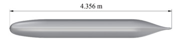Figure  8  Profile view of DARPA SUBOFF

Download: Full-Size Img

Table 7 compares the numerical and experimental results of Avci and Barlas (2018) for resistance (R_T), trim angle (τ), and sinkage($ \frac{\sigma}{L_{\mathrm{WL}}}$), with a corresponding Froude Number of 1.17. Uncertainty analysis of the resistance tests was conducted by Delen and Bal (2015) for the same model, estimating the total uncertainty in resistance to be 0.42%. Consequently, the validation uncertainty in R_T can be calculated as U_V = 3.1% according to ITTC (2017). In this study, the relative difference between experimental and numerical values of R_T is calculated to be 1.13%, indicating that validation is achieved within the validation uncertainty level. Additionally, the relative differences between the experimental and numerical results for trim and sinkage were found to be below the numerical uncertainty. Hence, validation is successfully achieved at the U_V level according to ITTC (2017).

Table 8 compares the numerical results with the experimental results of Roddy (1990) for the nondimensional drag force (X'). Roddy (1990) reported a total experimental uncertainty in X' of around 6%, which is greater than the relative difference between the numerical and experimental results. Therefore, validation is again achieved at the U_V level according to ITTC (2017).

3.2   Numerical ventilation

A well-known source of numerical error, particularly in CFD applications for high-speed surface ships, is the numerical ventilation (NV) error (Cui et al., 2021). This error mainly arises from the rotational motion of the body, leading to unintended air intakes below the hull due to numerical errors associated with the VOF method (GrayStephens et al., 2019). The presence of diffused air below the hull can markedly reduce drag; thus, special attention should be provided to avoid underestimating resistance.

Gray-Stephens et al. (2021) explored different methodologies to minimize NV. One effective approach was to introduce mesh refinement at the upstream side of the hull's bow. Another important strategy involves modifying the HRIC scheme to remove local CFL dependency (Bohm, 2014; De Luca et al., 2016). Thus, this study used the mesh refinement technique proposed by Gray-Stephens et al. (2021) alongside the modified HRIC scheme from Bohm (2014) to address the NV problem. Figure 9 compares the results obtained with and without NV treatment.

Figure  9  Volume fraction of water (Fr = 1.27)

Download: Full-Size Img

Table 9 compares the resistance values calculated with and without NV treatment. For all cases apart from Fr = 0.42, diffused air resulted in an underestimation in ship resistance. Additionally, the amount of the underestimation increases with ship speed.

3.3   Surface analysis

Figure 10 shows the wall y⁺ distribution around the hull at a speed of 30 kn. The calculated wall y⁺ values range from 60 to 100, which matches the log-law region of the turbulent boundary layer, where the normalized distance (y⁺) is expected to exceed 30 (ITTC, 2011).

Figure  10  Wall y⁺ Distribution Around the Hull (Fr = 1.27)

Download: Full-Size Img

Full-scale resistance results in kN relative to ship speed in kn are presented in Figure 11. Simulations were conducted over a speed range of 10–40 kn, with increments of ∆V = 5 kn. The total resistance at the design speed (V_A = 30 kn) is calculated to be 15.1 kN, corresponding to 233 kW of effective power.

Figure  11  Variation of the total resistance with speed

Download: Full-Size Img

Figures 12–14 show the ship's hull and the free surface elevation at different Froude numbers corresponding to transition or planing regimes. In the transition regime, where Fr ≤ 0.85, the ship generates a smooth wave with minimal spray, while the maximum amount of spray is observed at Fr = 1.06.

Figure  12  Profile view of the hull and surface elevation at different froude numbers

Download: Full-Size Img

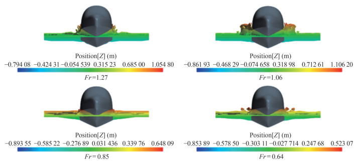Figure  13  Front view of the hull and surface elevation at different froude numbers

Download: Full-Size Img

Figure  14  Bottom view of the hull and surface elevation at different froude numbers

Download: Full-Size Img

Figures 15 and 16 show the variation of trim and sinkage with respect to the Froude number. The maximum trim value is calculated at Fr = 1.27, while the sinkage graph indicates that the hull generates substantial lift for Froude numbers of 1.06 or higher. All quantitative results for the at-surface simulations are given in Table 10.

Figure  15  Variation of trim with respect to Fr

Download: Full-Size Img

Figure  16  Variation of sinkage with respect to Fr

Download: Full-Size Img

3.4   Submerged analysis

Typically, semisubmersible naval ships operate in shallowly submerged conditions beneath the free surface. Their hydrodynamic characteristics, such as resistance, lift, and pitching moment, vary depending on the depth of submergence and the ship's speed. Simulations were performed with seven different depths (D), ranging from D/L_OA = 0.063 5 – 0.635, to evaluate the influence of the submergence depth. Two different speeds corresponding to Froude numbers 0.21 and 0.33 were used to investigate the effect of the ship's speed. In this study, submergence depth is defined as the vertical distance from the top end of the hull to the undisturbed free surface of the water, as schematically shown in Figure 17.

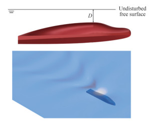Figure  17  Definition of the Submergence Depth

Download: Full-Size Img

The wall y⁺ distribution around the hull for Fr = 0.21 and D/L_OA = 0.254 is depicted in Figure 18. The y⁺ values are mostly in the range of 30–80, indicating that the centers of the cells adjacent to the hull surface fall within the inner log-law region of the turbulent boundary layer. This result shows the applicability of the wall functions.

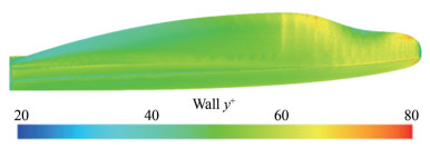Figure  18  Wall y⁺ distribution around the hull (Fr = 0.21, $ \frac{D}{L_{\mathrm{OA}}}$=0.254)

Download: Full-Size Img

Figures 19 and 20 show nondimensional hydrodynamic forces and pitching moments for Fr = 0.21 and Fr = 0.33, respectively, with quantitative results provided in Table 11. For both cases, the pitching moment values do not show notable changes with increasing depth. The M' values range from 0.000 7 to 0.000 8 for Fr = 0.21 and from 0.000 6 to 0.000 7 for Fr = 0.33. The results indicate that nondimensional pitching moment decreases slightly with increasing Froude number.

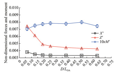Figure  19  Nondimensional forces and pitching moment (Fr = 0.21)

Download: Full-Size Img

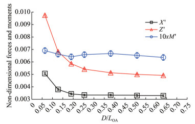Figure  20  Nondimensional forces and pitching moment (Fr = 0.33)

Download: Full-Size Img

Hydrodynamic lift and drag forces increase as operational depths decrease. This result is expected because pressure distribution around the hull generates a wave system when the ship operates near the free surface. The energy required to generate this wave system leads to an increase in drag and lift (Darrigol, 2005; Lighthill and Lighthill, 2001; Raphaël and De Gennes, 1966). In addition, lift and drag values increase according to the results.

Figure 21 shows the wave profiles calculated along the centerline of the hull for various operation depths. In contrast, Figure 22 compares the wave elevations for different Froude numbers. Notably, the figures reveal that vertical distance to the free surface and operating speed have considerable influence on the wave elevations. The hull generates substantially higher wave elevations when operating closer to the free surface and at higher speeds. Maximum normalized wave heights (H_max/L_OA) corresponding to various D/L_OA values are presented in Figure 23.

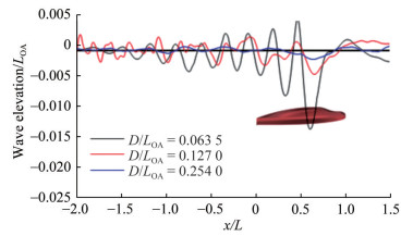Figure  21  Wave elevation at the centerline of the hull at operation depths ranging from D/L_OA = 0.063 5 to D/L_OA = 0.254 (Fr = 0.21)

Download: Full-Size Img

Figure  22  Wave elevation at the centerline of the hull at different froude numbers (D/L_OA = 0.063 5)

Download: Full-Size Img

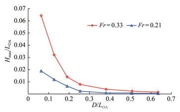Figure  23  Normalized maximum wave heights with respect to operating depths

Download: Full-Size Img

Figure 19 Nondimensional forces and pitching moment (Fr = 0.21) Figure 24 depicts the distribution of the dynamic pressure coefficient around the hull at six different depths of submergence, ranging from D/L_OA = 0.063 5 to D/L_OA = 0.635. Even at the highest depth of submergence (D/L_OA = 0.635), a low-pressure area appears above the hull before amidships due to the asymmetrical shape, generating upward lift. As the submergence depth decreases, this area shifts toward the after part of the hull, creating a wave trough above amidships, particularly when D/L_OA = 0.063 5. The reduction in pressure in this region causes higher hydrodynamic lift forces.

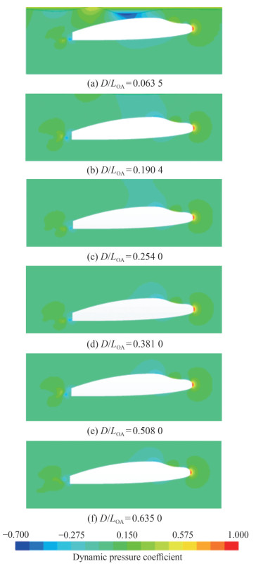Figure  24  Dynamic pressure distribution around the hull at various depth of submergence (Fr = 0.33)

Download: Full-Size Img

The hull was divided into 15 sections along the x-axis to determine the distribution of hydrodynamic lift, drag, and pitching moment along the length of the hull. The forces and moments acting on each part were calculated separately. Figure 25 shows the distribution of hydrodynamic forces and pitching moments along the hull for different operating depths. Hydrodynamic drag forces exhibit similar trends across all operating depths, with the magnitudes increasing as the depth of submergence rises, mainly due to the increase in hydrostatic pressure. The lift force distributions along the hull correlate with the pressure distribution (Figure 24). For all depths of submergence, low-pressure areas near amidships generate upward lift forces, while high-pressure areas toward the after part of the hull produce downward lift forces. Additionally, the pitching moment distribution along the hull follows a similar to that of the lift distribution, with the influence of submergence depth being more pronounced. Negative moment distributions are observed near the bow and aft of the hull, contributing to bow-down heave motion, while positive values are calculated around amidships where x/L_OA = 0.15 − 0.65, also contributing to the bow-down heave motion. The magnitudes of the nondimensional pitching moment coefficients increase with greater depths of submergence.

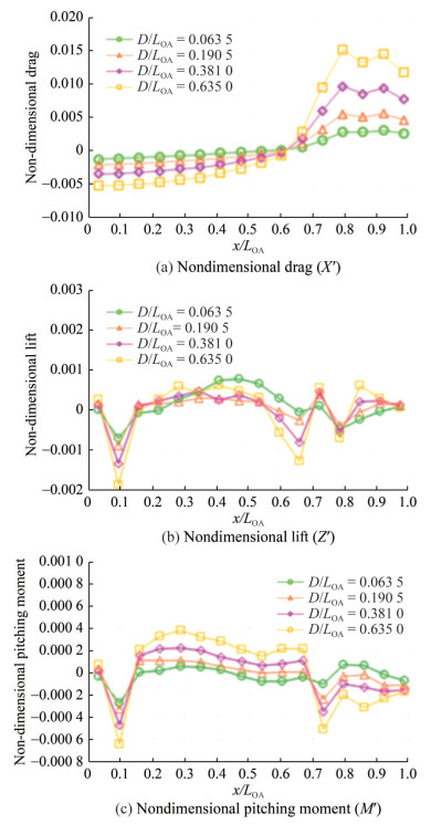Figure  25  Hydrodynamic force and moment distribution along the length of the hull (Fr = 0.33)

Download: Full-Size Img

4   Conclusions and future work

This article aims to investigate the hydrodynamic design features of semisubmersible naval ships, focusing on at-surface and shallowly submerged conditions. In this respect, two groups of simulations were conducted at full scale using a 15 m-long semisubmersible hull form. The study encompasses the resistance, powering, trim, and sinkage behaviors during at-surface operations, as well as the hydrodynamic lift, drag, and pitching moment during shallowly submerged operations.

The first group of simulations focused on at-surface resistance, powering, trim, and sinkage. All simulations were performed at full scale; thus, substantial numerical ventilation problems emerged, particularly at higher Froude numbers. These errors were minimized through upstream mesh refinement and the modified HRIC technique.

The total resistance of the hull was calculated as R_T = 15.1 kN at V_S = 30 knots design speed, corresponding to 233 kW effective power. A dynamic trim angle of τ = 1.40° was observed at this design speed. Low sinkage values were calculated when Fr ≤ 1.06. Notably, the hull generates substantial lift forces, and the draft begins to decrease when Fr > 1.06.

The second group of simulations focused on shallowly submerged conditions. These simulations mainly aimed to determine the hydrodynamic drag and lift forces, as well as the pitching moments at different depths of submergence. No direct relation between the pitching moment and submergence depth was observed. For both flow speeds, where Fr = 0.21 and Fr = 0.33, the pitching moment curve exhibited a similar trend with minimal changes depending on depth. Conversely, hydrodynamic lift and drag were found to be highly sensitive to the depth of submergence. Both force components acting on the hull demonstrated dramatic increases as the operating depth decreased. Additionally, nondimensional force coefficients increased, while nondimensional pitching moments slightly decreased with increasing Froude number.

The wave field above the ship has been shown to be significantly affected by the depth of submergence and the Froude number. Additionally, the pressure field near the hull surface plays a crucial role in the development of free surface elevations. This finding is particularly evident in the lowest depth case, where the low-pressure region above the hull around amidships leads to the formation of a wave trough, while the high-pressure region toward the aft creases a wave crest. The authors intend to conduct further experimental and numerical studies on the hydrodynamics of semisubmersible naval ships in future research.