1   Introduction

Rogue or extreme storm waves reach a height more than twice the size of those around them. In November 2020, a freak wave lifted a single buoy off the coast of British Columbia 17.6 m high; the four-story wall of water has now been confirmed as the most extreme ever recorded (NBC News, 2023). Although that wave was not the tallest, its relative size compared with the waves around it was unprecedented. However, a recent study predicted that wave heights in the North Pacific will only increase with climate change, which means that the 2020 wave may not hold the record for long.

The increased severity of extreme weather events associated with global warming has resulted in the increased occurrence frequency of marine accidents in the last years, as reported by Kharif et al. (2009) and Pilatis et al. (2024). Extreme sea conditions that involve waves with large amplitude to abnormal waves have consistently been an area of interest for naval architects. However, knowledge of the behavior of seagoing vessels in these extreme conditions remains limited due to the unavailability of real data and the complexity involved with the reproduction of such a large deterministic wave profile in a wave tank. For the same reason, the validation of numerical codes in extreme sea conditions remains restricted.

Seakeeping analysis has been made possible by the development of numerical methods with various levels of complexity, which vary from linear strip theory solutions to complex computational fluid dynamics (CFD) codes (Parunov et al., 2022). Ship responses in extreme seas exhibit a high nonlinearity, which mainly originates from two sources, i.e., free surface and geometry of the ship. The classic linear methods, e.g., those proposed by Guedes Soares and Schellin (1998) and Clauss et al. (2010), cannot provide accurate predictions for responses of ships with large bow flare angles as reported by Fonseca and Guedes Soares (2004a, 2004b). The commonly known techniques for dealing with free surface nonlinearity include weakly and fully nonlinear numerical solutions. The partially nonlinear time domain method (Fonseca and Guedes Soares, 1998a, 1998b), where Froude–Krylov and hydrostatic-related forces are nonlinear, was validated for predictions of responses to abnormal waves (Guedes Soares et al., 2008; Fonseca et al., 2010). However, the sagging moment peaks in very large and steep waves are overestimated (Rajendran et al., 2011, 2012). Through the inclusion of body nonlinearities in radiation and diffraction forces, Rajendran et al. (2015) reported good predictions on vertical motions and loads of a cruise ship subject to large amplitude waves. Various nonlinear time-domain codes were compared by Watanabe and Guedes Soares (1999) to predict vertical bending moments (VBMs) in a containership. A good agreement was obtained among the computed values for low wave heights. However, high deviations were detected in the higher-wave region, where the elastic behavior of the hull played a crucial role. Holloway and Davis (2006) discussed high-speed strip theories, where the time-domain high-speed theory was recommended as a practical alternative to three-dimensional (3D) methods. Bhatia et al. (2023) conducted systematic comparative research on the investigation of the ship's pitch, heave, and roll movements in irregular waves using strip theory.

The 3D boundary element method (BEM), which uses either a Green's wave function (Zakaria, 2009; Sengupta et al., 2016; Datta and Guedes Soares, 2020; Negi et al., 2022) or a Rankine source (Yasukawa, 2003; Guo et al., 2013; Yao et al., 2019) is a good tool for the estimation of nonlinear ship responses in low to moderate seas. However, further investigations still need to be conducted to determine their capability to predict ship responses in extreme situations. CFD codes based on Navier–Stokes equations are considered the highest level of complexity method that can include most nonlinearities, including fluid compressibility, viscosity, and cavitation (Wang and Guedes Soares, 2020; Wang et al., 2021; Zhang et al., 2023). Various CFD solvers for the prediction of ship behavior in waves have been validated against experimental or other numerical solutions, e. g., those introduced by Oberhagemann et al. (2012), Simonsen et al. (2013), Chen and Chen (2014), Jiao et al. (2021), and Kudupudi et al. (2023). Phan and Sadat (2023) conducted CFD simulations of extreme ship responses by designing wave trails for a KRISO container ship (KCS) advancing at Fn = 0.26. The wave trails designed under the non-Gaussian process provided the desired response except for the heave response of 0.2 m.

However, in addition to high computational expenses, various uncertainties, such as the discretization error (Wang et al., 2022) or modeling uncertainty from the turbulence model (Xiao and Cinnella, 2019), affect the accuracy of numerical modeling. To ensure the accuracy of numerical solutions, scholars have focused on uncertainty quantification. Uncertainty analysis usually includes two steps, namely verification and validation (ITTC, 2008; ITTC, 2017). Verification refers to the process of determining whether a model implementation accurately represents the implemented algorithm and model solution. Validation indicates the determination process of the degree to which a model prediction adequately represents measured physical phenomena through their comparison with the findings observed in experiments.

Drummen and Holtmann (2014) presented a benchmark of uncertainties that relate to slamming and whipping analysis, and the results showed that uncertainties in wet frequencies may be lower compared with those relevant to dry modes. The damping coefficient affected the results considerably. Kim and Kim (2016) applied total difference in a benchmark study to assess the deviation of an individual numerical model against the means of all models of the predictions of motions and loads of a 6750-TEU containership. Abdelwahab et al. (2023) reported a new model of uncertainty measure for wave-induced motions and loads. Qiu et al. (2019) presented extensive experimental benchmark data and conducted a detailed uncertainty analysis of the findings of two-body interaction model tests. Quantification of uncertainties in model geometry, model mass properties, locations of models, and setup of the mooring system was performed. The uncertainties due to model geometry were negligible, but those resulting from the model mass properties may be crucial for roll motions. The uncertainty in the gap led to large uncertainties in all measured results. Parunov et al. (2020) presented an experimental benchmark and uncertainty assessment study organized by the MARSTRUCT Virtual Institute on global linear wave loads on a damaged ship; the study emphasized the unaccounted uncertainty in measurements. The review of Hirdaris et al. (2023) further confirmed the importance of uncertainties in the modeling and validation of wave loads for ship design development and assessment. The benchmark on the prediction of the whipping response of a warship model in regular waves (Parunov et al., 2024) revealed the similarity of uncertainty in rigid body response to that in previous analysis; however, whipping responses revealed considerable differences among approaches, which were mainly caused by slamming simulation. The differences arise not only from the models that calculate the elastic response of the structures but also from the models that quantify the slamming loads (Wang and Guedes Soares, 2017).

The ISSC-ITTC Joint Committee organized a benchmark study (Parunov et al., 2022) on global linear wave loads on a container ship with forward speed to assess uncertainties in linear transfer functions resulting from various seakeeping codes and consequences on long-term extreme vertical wave bending moments. The study confirmed the substantial differences between methods based on the same mathematical model and recommended the initiation of benchmark studies on various ship types to provide a basis for the quantification of uncertainties. To provide a database as the potential benchmark study, Klein et al. (2023) presented experimental data on the ship motions and wave- induced loads of an LNG carrier in extreme seas from the EU project EXTREME SEAS. This study aimed to provide a comprehensive discussion on the behavior of a chemical tanker (CT; from the same project) in extreme waves and provide additional information on benchmarks of various ship types.

2   Description of model tests

Model tests on the CT were conducted in the seakeeping basin of the Ocean Engineering Division of the Technical University Berlin. The basin measures 110 m in length, with a measurement range of 90 m, 8 m in width, and 1 m in water depth. One side is installed with an electrically driven piston-type wave generator. The wave generator is fully computer-controlled, and the implemented software enables the generation of transient wave packages, deterministic irregular sea states with definite characteristics, and tailored critical wave sequences. The opposite side is installed with a wave-damping slope to suppress wave reflection.

2.1   CT model

The investigated CT model comprised a fiberglass-reinforced plastic at a model scale of 1:70. Table 1 presents the main dimensions, and Figure 1 displays a side view sketch of the CT with the coordinate origin for all subsequent position specifications. Table A1 in Annex A provides the detailed mass distribution, including the moment of inertia and center of gravity of the individual mass.

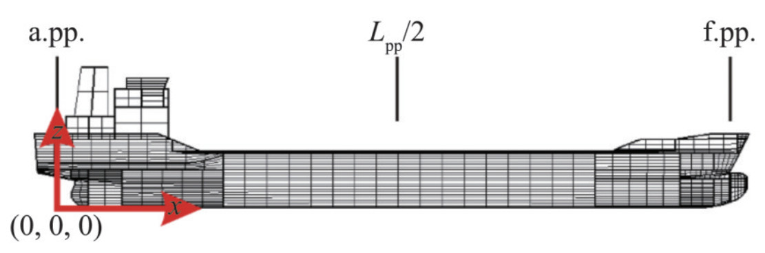Figure  1  Coordinate system of the investigated CT

Download: Full-Size Img

2.2   Model equipment and test setup

The model tests were conducted to measure global ship motions, global and local loads, and the wave profile on the weather deck at the bow. For these purposes, the model was equipped with various sensors, hardware for data acquisition (a small computer, amplifier, analog-to-digital converter and measurement card) and power supply for self- sufficient tests, i. e., all sensor data from sensors on the ship were collected onboard. Thus, only one cable, which served as a trigger for time synchronization, was connected to the main control and measurement system. The main system was used to control the wave maker and measure surface elevation at various wave gauges and ship motions. The test setup comprised the suspension system that held the model in position during the tests, the tracking system that measured absolute motions, and the wave gauges that measured the encountering waves.

2.2.1   Pressure transducers

The model was instrumented with pressure transducers at various positions on the hull: on the bow, on deck at the forecastle area, and on the keel near the bow and at the stern. Figure 2 illustrates the pressure transducer locations at the bow (Figure 2(a)) and stern (Figure 2(b)). The model was used with a focus on the time series of pressure loads on the bow due to steep large waves. Therefore, a large area at the bow of the vessels was equipped with pressure transducers to obtain information on the local pressure distribution on the bow and the associated global effects on VBMs. Annex B provides a detailed discussion of the position of pressure transducers and their measurement characteristics and uncertainties.

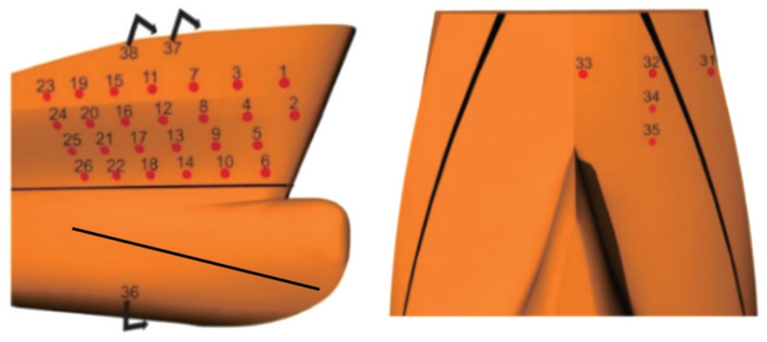Figure  2  Overview of pressure transducer locations

Download: Full-Size Img

2.2.2   Force transducers

The ship model was divided into two segments at L_pp/2 and connected to three force transducers for global load measurement, particularly the vertical wave bending moment. The deck of the ship model was mounted with two force transducers, with one being positioned underneath the keel. The force transducers, which had a nominal load of 200 kg and a protection class of IP68 (100 h at 1 m water column), registered the longitudinal forces from which vertical wave bending moments and longitudinal forces were calculated based on a given geometrical arrangement. On this basis, superimposed vertical wave bending moments, including the counteracting VBM caused by longitudinal forces with respect to selected vertical levels, were determined.

2.2.3   Green water gauges

In addition to two pressure transducers (PT 37 and 38) mounted on the deck, two green water gauges (with absolute and measurable green water heights on the deck of 0.192 and 0.133 m) were installed at the same longitudinal positions. Figure 3 illustrates the positions and dimensions. The height of the forecastle level was approximately 45 mm.

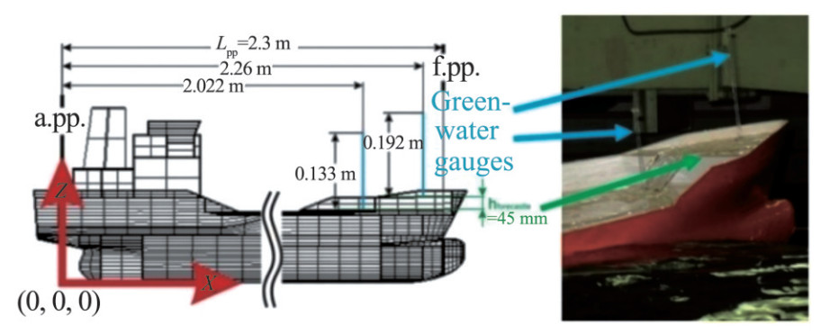Figure  3  Positions and dimensions of green water gauges

Download: Full-Size Img

2.2.4   Suspension system

The model tests involved fixing the model with an elastic suspension system using a triangular towing arrangement, which pulled the model without inducing a moment (Klein et al., 2023). A spring in front of the model and a counterweight behind it restricted the longitudinal motions. With this arrangement, heave and pitch motions and the measured forces and moments remained unrestrained.

2.2.5   Absolute motions

An optical tracking system recorded ship motions. The tracking system comprised a ceiling frame equipped with five infrared cameras, which were shifted parallel to the moving ship model. The system enabled high precision, contact-free motion tracking over large distances by following the trajectories of infrared light-emitting diodes mounted on the ship model.

2.2.6   Wave gauge positions

The number of wave probes varied based on the objective of the test campaign. Figure 4 illustrates the wave gauge positions in the model tests in stationary conditions. Altogether, nine wave gauges were installed, with the first one placed at 6.2 m in front of the model at xt1 = 39.9 m. A cluster of seven gauges, separated at s = 0.1 m intervals, was arranged around the target location to investigate the spatial evolution of waves at the bow.

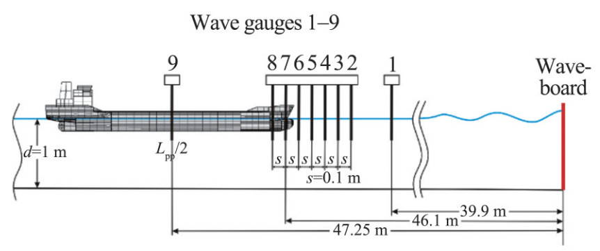Figure  4  Sketch of the wave gauge positions

Download: Full-Size Img

Furthermore, one gauge was installed amidships. For the ship with a forward speed of Fn = 0.08, this setup was reduced to three wave gauges, with one placed at 6 m in front of the forward perpendicular (gauge No. 1 in Figure 4), one at the forward perpendicular (gauge No. 7 in Figure 4), and another amidships (gauge No. 9 in Figure 4) relative to the idle state of the model.

3   Experimental program and results

The experimental program focused on investigating the frequency and time domain. One goal of the model experiments was to determine behavior in the form of transfer functions. Therefore, the model was investigated via the transient wave packet (TWP) technique to obtain the response amplitude operator (RAO), and the results were evaluated via tests involving regular waves of various steepness. The model was also investigated in irregular waves, critical wave sequences, real extreme wave reproductions, and breather- type extreme waves. The following subsections present the various parts of the experimental program.

3.1   TWP

The TWP technique serves as an efficient method for the determination of the sea state behavior of ships and floating structures and the RAO in one test run (e. g., Clauss and Kühnlein, 1995, 1997; Clauss and Steinhagen, 1999; Clauss et al., 2010, 2014; Klein et al., 2021). TWPs comprise synthesized task-related wave spectra with tailor- made phase distribution, and they can be easily adapted to the relevant frequency range of interest.

Figure 5 presents the test results on TWP measurements (blue curves) compared with numerical simulations (red curves). Numerical simulations were performed with the use of an established frequency domain program (Wave Analysis at Massachusetts Institute of Technology (WAMIT)) for comparison. WAMIT is a radiation/diffraction program that evaluates wave-structure interaction at zero speed in the frequency domain (Newman, 2018; WAMIT, 1994; Lee, 1995); this program is a widely accepted and validated numerical tool for hydrodynamic analysis and suitable for a multitude of applications.

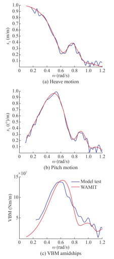Figure  5  Comparison of measured (blue curves) and calculated RAOs (red curves)

Download: Full-Size Img

For the VBM RAO, the agreement between experimental results and WAMIT was only sufficient as a distinct shift was identifiable. The detailed reason for the shift was indeterminable but is in line with the findings of other numerical tools (Ley and el Moctar, 2021; Guedes Soares et al., 2006).

3.2   High and steep regular waves

To identify the influence of wave height and steepness on the VBM, model tests on regular waves of various wavelengths and steepness were performed. Regarding the dependence of the ship length, different relative wavelengths (wavelength/ship length) with varied crest/trough asymmetries were selected to evaluate the influence of wave steepness on VBMs. The investigated discrete regular wave lengths (L_w) were selected to cover the complete range of interest in the frequency domain, i. e., from L_w/L_pp = 0.6 to L_w/L_pp = 2.2. For the evaluation of wave steepness influence, the test program was divided into two parts, with each part having the same wavelengths with varying wave steepness. Wave height and steepness were selected in such a manner to obtain wave profiles with various crest/trough asymmetries and evaluate the influence of unique wave profiles (asymmetries) on VBMs.

Figure 6 illustrates the regions of validity of wave theories on wave profiles and the selected wave steepness and wavelengths of the experimental program. The relative water depth and wave height were plotted on the abscissa and ordinate, respectively. The first part of the experimental program included regular waves with moderate amplitudes (0.002 ≤ H/(g·T²) ≤ 0.004), where the wave profile was within the Stokes Ⅱ domain (cf. Figure 6-red dots). The second part of the test campaign involved the generation of the same (regular) wavelengths but with increased relative wave heights (0.01 ≤ H/(g·T²) ≤ 0.012, where the wave profile was within Stokes Ⅲ domain (cf. Figure 6, blue dots).

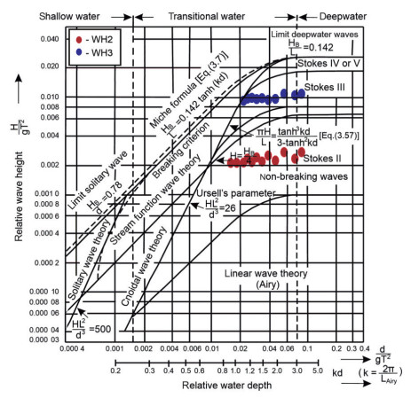Figure  6  Breaking wave height and regions of validity of various theories on gravity water waves (Clauss et al., 1992)

Download: Full-Size Img

Figure 7 presents the test results on regular waves, including the respective RAOs (|sagging moment| + hogging moment-red dashed curves) compared with the TWP RAO (black curves). The sagging (red crosses- (2· |M_sagging|/H)) and hogging moments (red circles- (2·M_hogging/H)) were additionally registered to evaluate the asymmetry of measured bending moments compared with the wave steepness. M_sagging and M_hogging refer to the minimum and maximum vbm, respectively, i. e., the negative and positive amplitudes of the measured time series in different regular waves.

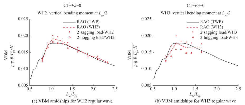Figure  7  Comparison of the RAO for the VBM at L_pp/2 determined via the TWP technique and the results on regular waves

Download: Full-Size Img

The results on RAOs obtained in regular waves (red dashed curves) and with the TWP (black curves) showed a generally good agreement. However, the increase in the asymmetry between hogging and sagging moments with the increase in wave steepness was identifiable and followed those of previous investigations (Fonseca and Guedes Soares, 2002; Clauss et al., 2010). In addition, the VBM trend for the WH3 regular wave results displayed a distinctive feature, which was unexpected at first glance: the overall VBM obtained with the WH3 regular waves (red dashed curve) was below the RAO acquired through the TWP technique. This finding does not denote shrinkage of the VBM shrunk. Instead, the RAO value decreased proportionally to the wave height. This effect can be attributed to the small freeboard height of the CT compared with the large wave height, with parts of large wave crests spilling over the deck in terms of green water instead of acting on the bow, which resulted in a smaller VBM-to-wave height ratio. Furthermore, additional effects due to the influence of the shipping of water on deck, which affect ship motions (Fonseca and Guedes Soares, 2005) and induce a counteracting moment due to the green water mass on deck (Clauss et al., 2010; Rajendran et al., 2011), may be considered.

3.3   Irregular sea states with random phases

Several irregular sea states were investigated in model tests representing design storms in accordance with existing probabilistic methods. These sea states, each lasting 30 min in real time, are presented in Table C1 in Annex C. Each characteristic sea state parameter set was used to generate up to six wave sequences having the same T_p, H_s, and ɣ but various random phase seeds for long-term statistical analysis. The phases were randomly generated and varied within each parameter set but were constantly plugged for each one. Parameter set No. 1 (Table C3), phase seed #1 had another random phase distribution than phase seed #2, #3, and so on of the same set but the same phase seed such as set No. 2, phase seed #1, set No. 3, phase seed #1, and so on. Altogether, 45 runs were conducted under stationary conditions (Fn = 0) and at forward speed (Fn = 0.08).

Figure 8 presents the comparison of the time series of the wave surface elevation at L_pp/2, heave, pitch, and VBM at L_pp/2 between experimental measurements and numerical predictions from the work of Rajendran et al. (2015) for the CT with zero forward speed. The sea state IRREGULAR20 with T_p = 12 s and H_s = 11.5 m with phase seed #1 was used. The wave surface elevation showed good agreement, which indicates that the numerical approach reproduced the wave surface sequences very well. The motion and loads agreed well, although the peaks exhibited slight deviations. The experimental results on heave and pitch motion transpired slightly earlier than numerical predictions. This phase shift was attributed to the suspension systems applied in the tests to maintain the model in position as the ship model generally shifted backward due to waves and oscillated around a new dynamic position. Another reason for the discrepancies was the assumption made in the numerical method, which disregarded the interaction between the incident wave field and the ship hull. Typically, this interaction resulted in a wave run-up as the waves encountered the hull, which led to further differences between experimental and numerical findings.

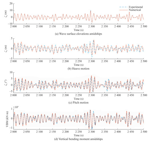Figure  8  Comparison of the numerical prediction of the time series of the wave surface elevation at midships, heave, pitch, and VBM with those experiments using the sea state IRREGULAR20 phase seed #1 when Fn = 0

Download: Full-Size Img

Figure 9 shows the comparison of the exceedance of probability of the maxima and minima of the wave elevation, motions and loads in the sea state IRREGULAR20 phase seed #1. Consistent with the time series, the peaks of wave surface elevation showed excellent agreement. For heave and pitch motions, the positive peaks from numerical predictions were slightly higher, and the negative peaks were in good agreement for small values but were slightly lower for extreme values. As for the VBMs at L_pp/2, the numerical approach overpredicted the hogging and sagging peaks in general, although the maximum values in hogging were a bit lower than the measurements. The comparisons between the numerical predictions and the measurements were similar to those for the LNG in the work of Klein et al. (2023).

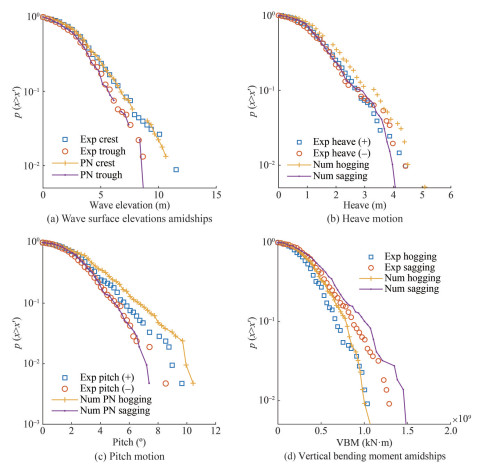Figure  9  Comparison of the exceedance of probability of the maxima and minima of the time series of motions and loads in the sea state IRREGULAR20 phase seed #1 when Fn = 0

Download: Full-Size Img

To study the experimental uncertainties in the model tests, we performed statistical analysis of the measurements in the same sea states but with various phase seeds. Figure 10 presents the exceedance of the probability of the peaks for the wave surface elevation, motions, and loads of the CT in IRREGULAR20 conditions from five repeated model tests with different phase seeds. When the values of peaks were small, the five tests provided almost the same exceedance probabilities, whereas slight deviations were observed for the calculations on higher peaks. In particular, the highest deviations were found in the peaks from run 1 (seed #1).

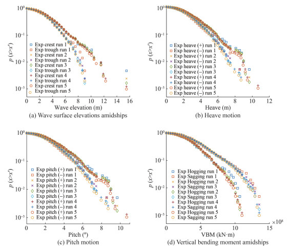Figure  10  Exceedance probability of peaks for the motions and VBM in sea state IRREGULAR20 of all five phase seeds when Fn = 0

Download: Full-Size Img

For quantification of experimental random uncertainties, the statistical values, e.g., the means of all the peaks, the 1/3 largest peaks, and the 1/10 largest peaks, were calculated for all the five runs, and random uncertainties were presented as percentages relative to the mean values of the five runs. Table D1 in Annex D lists all random uncertainties of wave surface elevation, heave, and pitch motions and VBM at L_pp. Except for the random uncertainty for the mean of the 1/10 largest peaks of the heave trough (1.8%), the uncertainties for all other metrics were lower than 1%, which is considered low.

The wave-induced pressures at the bow and stern of the CT were also measured in the model tests. The comparison the numerical prediction and experimental data on the pressures can be found in Wang and Guedes Soares (2016a, 2016b). Figure 11 shows the part of the time series of pressures at the bow (Pressure transducer #02) and stern (Pressure transducer #32), together with the identified peaks. Given the small draft at the stern, the identified peaks were more than those at the bow. The probabilities of exceedance for the identified pressure peaks were compared (Figure 12) for the five phase-seeds when the ship's forward speed was zero. The deviations of pressure peaks between the five runs were larger than the motions and the VBM, in particular for those from pressure sensor #32.

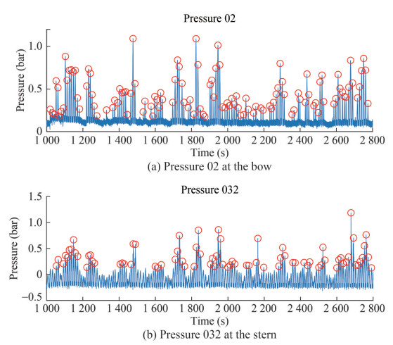Figure  11  Time series of the pressure at the bow and stern of the CT in sea state IRREGULAR20 phase seed #1 when Fn = 0

Download: Full-Size Img

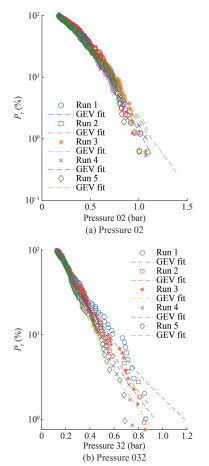Figure  12  Exceedance probability for the pressure peaks in sea state IRREGULAR20 for all five runs when Fn = 0

Download: Full-Size Img

Figure 13 shows the probability of exceedance for the pressure peaks when Fn = 0.08. The deviation was lower compared with that when Fn = 0, in particular for the smaller peaks. To quantify the experimental random uncertainties for the pressures, we also calculated the statistical values for the five phase seeds. The random uncertainties are listed in Tables D2–D3 when Fn = 0 and Fn = 0.08, respectively, where the extreme values (probability equals 1%) were estimated using the generalized extreme value (GEV) analytical distribution model by fitting the identified peaks. The maximum uncertainty occurred at the extreme value for the case pressure No. 02 with Fn = 0. When Fn = 0.08, the maximum uncertainty was the largest at the mean value of the 1/10 largest peaks. These results are consistent with the values in Figures 12 and 13, where high deviations were observed at low probability. All uncertainties at pressures were lower than 10.5%, and the forward speed of the ship did not cause a considerable increase in the uncertainties on the pressure at the bow.

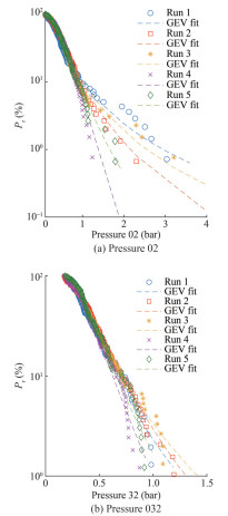Figure  13  Exceedance probability for the pressure peaks in sea state IRREGULAR20 for all five runs when Fn = 0.08

Download: Full-Size Img

3.4   Extreme wave events

The investigation of extreme wave events is essential for the thorough assessment of ships. In addition to the statistical determination of extreme responses through investigations of irregular sea states with predefined design wave spectra and random phase distributions, the exploration of deterministic extreme wave sequences enables the deterministic evaluation of critical wave sequences and extreme responses. Specifically, experiments on deterministic extreme wave events enable the detailed analysis of the cause-and- reaction chain concerning specific research questions. This approach allows for the evaluation of whether such wave events are critical for the investigated structure, a dimension not covered by statistical analysis.

The investigations on extreme wave events encompass real measurements and the study of specific design extreme wave groups. The renowned Draupner wave, also known as the "New Year's wave" (NYW) (Slunyaev et al., 2005; Cherneva and Guedes Soares, 2008), was recreated in the seakeeping basin to provide a real-world replication. For the generation of extreme design wave groups, exact solutions of the nonlinear Schrödinger equation (NLS), known as breather solutions, were employed. These breather solutions exhibit quasimonochromatic waves that experience slight disturbances in time or space. The modulation instability leads to an escalated disturbance during development, which results in a considerable amplification of the original amplitude. Three types of breather solutions were utilized in total: the Kuznetsov–Ma (Kuznetsov, 1977; Ma, 1979), Akhmediev (Akhmediev et al., 1985; Akhmediev and Korneev, 1986; Akhmediev et al., 1987) and Peregrine breather (Peregrine, 1983). These breather solutions were assessed for their suitability in addressing research questions related to the effects of extreme waves.

The utilization of breather solutions for model tests offers several advantages. One notable aspect is their straightforward applicability in designing extreme waves. According to Klein et al. (2016), "The major benefits include the potential to generate abnormal waves of a certain frequency up to the physically possible wave height, the symmetrical shape of the extreme wave, and the availability of an analytical solution." This analytical solution facilitates the rapid and uncomplicated generation of wave maker control signals.

Notably, breather solutions, particularly the Peregrine breather, are considered a unique prototype of extreme waves (Shrira and Geogjaev, 2010). Wang et al. (2016) have demonstrated the applicability of the Peregrine breather for modeling extreme waves in realistic oceanic conditions. Such a result was achieved by embedding the Peregrine breather in complex sea states based on JONSWAP spectra. In alignment with this outcome, experimental findings by Klein et al. (2016) reveal the possibility of incorporating Peregrine breathers into irregular sea states to create tailored extreme wave sequences. Moreover, such designed extreme waves exhibit dynamics similar to the real-world Draupner wave.

Next, experiments on the Peregrine breather solution were presented exemplarily and compared with the results on the Draupner wave. Klein et al. (2023) reported the application of all three breather solutions in model tests in extreme waves. The Peregrine breather solution was used to generate a set of high, steep single waves of various discrete carrier wavelengths to cover the range of interest in the frequency domain covering the VBM. The initial steepness at the wave board was defined in such a manner as to guarantee that a single wave at the target location is as high as physically possible for the defined wavelengths.

3.4.1   Breather-type extreme waves—Peregrine breather

The Peregrine breather solution (Peregrine, 1983), also known as a rational solution, represents the limiting case of the time-periodic Kuznetzov–Ma breather and space- periodic Akhmediev breather. Specifically, this solution is neither temporally nor spatially periodic: it is a wave that "appears from nowhere and disappears without trace" (Akhmediev et al., 2009) and is considered a special prototype of freak waves (Shrira and Geogjaev, 2010).

The Peregrine breather solutions applied in the experiments represent an exact solution of the NLS equation:

For the wave group evolution in the space of a time series, with

and

The coefficients and read for arbitrary water depth are as follows (Serio et al., 2005):

where k_c represents the carrier wave number, ω_c denotes the corresponding angular frequency, C_g refers to the group velocity, and d is water depth. The correction for the group velocity in finite water depth is considered using the coefficient ν:

The analytical form of the Peregrine breather solution suitable for wave tank experiments is given in the following equation (Karjanto and van Groesen, 2007):

with

In general, full determination of the Peregrine solution in space and time requires predefined plane-wave amplitude a_c and carrier frequency ω_c (i.e., initial steepness).

3.4.2   Experimental results

The CT was investigated in the Peregrine breather solution introduced above to evaluate the effect of such a high, steep single wave. Initially, a series of high, steep single waves with various discrete carrier wavelengths was generated using the mentioned solution. These carrier wavelengths were selected to span the frequency domain of interest for the VBM in the range of L_w/L_pp = 0.8 to L_w/L_pp = 1.5. The initial steepness at the wave board was determined, and as a consequence, the high single wave at the target location reached the maximum wave height physically possible for the specified wavelengths.

The calculated waveboard surface elevation served as the basis for control signal generation. The theoretically predicted location of the extreme wave occurrence (input) and registrations/observations in the tank demonstrated satisfactory agreement. In most cases, the actual extreme wave event closely matched the given value. However, as wave-structure investigations necessitate the definition of target waves in the time domain at precise locations, the examined breather-type extreme waves presented here resulted from the adjustment of the first control signal to accurately achieve an extreme wave at the target location. For this adjustment process, up to three iteration steps were considered.

Figure 14 illustrates the outcomes of model tests conducted under stationary conditions (Fn = 0) in Peregrine breather extreme waves from the top (the shortest) to the bottom (the longest wavelength). The CT was investigated in four carrier wavelengths (L_w/L_pp = 0.8 to L_w/L_pp = 1.5). A trio of diagrams was used to present the findings for each carrier wavelength. The upper diagram displayed the surface elevation at the forward perpendicular, the middle diagram the VBM amidships, and the lower diagram the green water column height on the deck at the forward perpendicular. The design vertical wave bending moment following the IACS-Common Rules (IACS, 2015) was also presented to assess the measured VBM. During the dimensioning process of the transverse section, additional parameters, such as γR, cs, deck openings, etc., must be considered. The design vertical wave bending moment is represented by black dashed lines. The diagrams also show the ultimate design vertical wave bending moments, calculated based on the design VBM while considering safety factors.

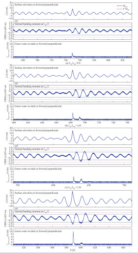Figure  14  Results of the model test in Peregrine breather extreme waves

Download: Full-Size Img

The presented findings reveal that the distinct single wave was prominently visible at the forward perpendicular across all wavelength-to-ship-length ratios. The height of extreme waves shown increased proportionally with the carrier wavelength because all the presented waves were deliberately generated to achieve the highest physically possible wave height at the targeted location, which resembles a plunging breaker in proximity.

Similar to the outcomes noticed in regular waves, the resulting VBM was influenced by wavelength and attained maximum values at critical wavelengths corresponding to the wave height. However, the absolute values were notably elevated due to the influence of the highest physically possible wave height, which is in contrast to those of tests on regular waves featuring moderate wave steepness. The wave heights of the highest and steepest regular waves (WH3) were roughly 40% smaller compared with the Peregrine breather. A comparison of absolute VBM values indicates that the moments were at least 15% higher for hogging conditions and 30% higher for sagging conditions than those measured in regular waves. The maximum VBM, particularly in sagging moments, exceeded the design vertical wave bending moment and nearly reached the ultimate design wave bending moment. Although this excessive design vertical wave bending moment did not necessarily lead to an inevitable structural failure of the ship at full scale—given that additional parameters must be considered for transverse section dimensioning—it underscored the severity of the impact of Peregrine breather extreme waves, which constitutes a limiting case for the investigated ship.

This severity was further corroborated by the measured green water column heights at the forward perpendicular, which attained impressive values. A wavefront of 10 m in height, an elevation as tall as a single-family home, was detected spilling over the deck at the forward perpendicular.

Parts of the time series of slamming pressures were compared with those of the model tests in breather-type extreme waves with L_w/L_pp = 0.8 to L_w/L_pp = 1.5 (Figure 15) with the results at the bow (pressure sensors No. 02) and stern (pressure sensors No. 32). Comparison with the time series of the wave surface elevation in Figure 14 indicated that for all presented pressure sensors, the maximum value occurred after the highest wave impacted the hull. The maximum pressure peaks from sensor No. 02 for L_w/L_pp = 0.8 (Figure 15(a)) were 0.65, 0.64, and 0.64 bar, for the Peregrine breather, Ma–Kuznetsov breather and the space-periodic Akhmediev breather extreme waves, respectively. The values were 0.78, 0.89, 0.92, 0.86, 0.87, and 1.07 bar for L_w/L_pp = 1.05 (Figure 15(b)) and 1.28 (Figure 15(c)). Thus, at a higher ratio of L_w/L_pp, the pressure peaks were larger. In general, the space-periodic Akhmediev breather extreme waves provided slighter higher pressure, but the deviations between the three types of waves were small.

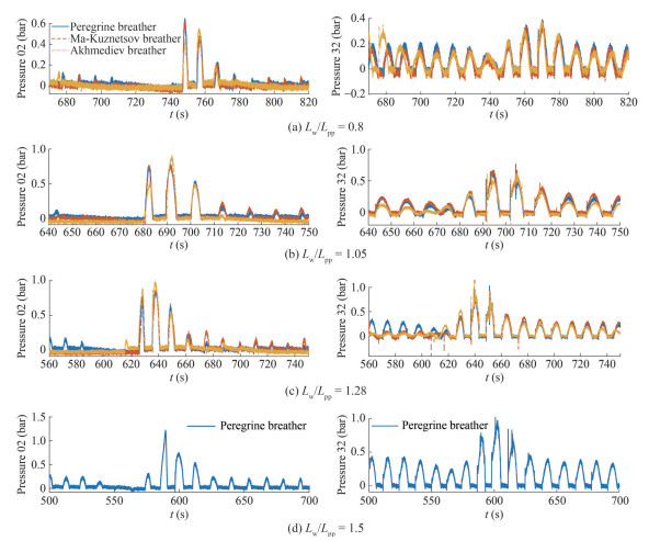Figure  15  Results on the pressures at the bow and stern from model tests in breather-type extreme waves with L_w/L_pp = 0.8 to L_w/L_pp = 1.5

Download: Full-Size Img

As for the pressures at the stern (sensor No. 32), the maximum peaks were lower overall compared with those at the bow. However, when the ratio of L_w/L_pp increased, the differences became smaller. High slamming pressures were captured at the bow and the stern of the model for L_w/L_pp = 1.5. As displayed in Figure 15(d), the maximum pressures were 1.22 and 1.02 bar, respectively. Through the GEV distribution, the most probable extreme values of the peaks on pressure sensors No. 02 and No. 32 reached 1.02 and 0.74 bar for the case in sea state IRREGULAR20 with H_s = 11.5 m and T_p = 12 s and with zero forward speed. In particular, the peaks of the Peregrine breather L_w/L_pp = 1.5 case were 20%, 37% and 58% higher than the extreme values.

Altogether, the results indicate the Peregrine breather solution as a powerful tool for the generation of tailored extreme waves having certain critical wavelengths, which will enable the investigations of limiting cases on various subjects, e. g., local and global loads, green water effects, and air gap investigations (Klein et al., 2016).

3.4.3   Real-world extreme wave reproduction

To assess the outcomes of the model tests utilizing the breather solutions, we subjected the CT to a real-world extreme wave replication—the famous Draupner wave. On January 1, 1995, the Draupner extreme wave was documented during a storm at the Draupner platform in the North Sea. A giant single wave (H_max = 25.63 m) with a crest height of ζ_c = 18.5 m formed in a surrounding sea state, and it was characterized by a remarkable wave height of H_s = 11.92 m (H_max/H_s = 2.15). The location had a water depth of d = 70 m. Figure 16 shows a comparison of the measured model wave train at the target position and the full-scale recorded sequence at the Draupner platform. The highest wave generated in the tank matched well with the real-world one. Given the complex reproduction of such steep wave groups due to strong nonlinearity, the NYW was reproduced in accordance with an optimization procedure (Clauss and Klein, 2011) that focused on the reproduction of the target wave as exactly as possible. As a result, the surrounding wave groups differed from real-world measurements.

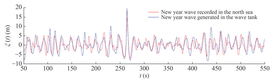Figure  16  Comparison of measured model wave train at target position and the recorded sequence in the Draupner platform (full scale)

Download: Full-Size Img

Figure 17 illustrates the outcomes for the CT under stationary conditions (Fn = 0) in the Draupner wave. Figure 17(a) presents the surface elevation at the forward perpendicular, Figure 17(b) depicts the corresponding VBM, and Figure 17(c) shows the green water on the deck at the forward perpendicular. The findings obtained in the Draupner wave (depicted by blue curves) were juxtaposed with those measured in the Peregrine breather (represented by red curves) with L_w/L_pp = 1.3 (Figure 14). The selection of this wave sequence was due to the nearly the same exceptionally high wave crest height of extreme waves at the target location. However, the Peregrine breather was also distinguished by deep preceding and following troughs and short up- and downcrossing wave periods. Thus, a high and steep Peregrine breather was observed.

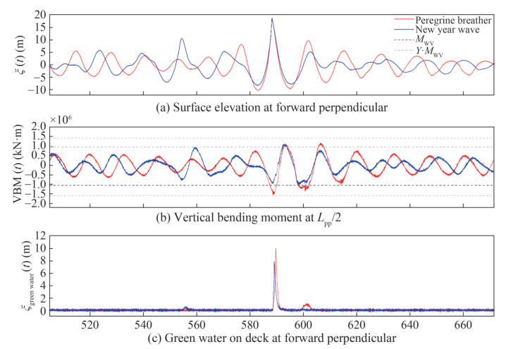Figure  17  Results of the model tests in the Draupner wave vs. Peregrine breather extreme wave

Download: Full-Size Img

Comparison of the recorded loads (Figure 17(b)) and the green water column on the deck (Figure 17(c)) showed that the Draupner wave and the Peregrine breather extreme wave pose substantially impacted the ship. In the case of the Draupner wave impact, the measured VBM reached the design vertical wave bending moment, and the green water column height on deck was notably impressive at approximately 8 m. However, the impact of the Peregrine breather was more severe, which resulted in higher hogging and sagging loads and a greater green water column height on deck.

This discrepancy was primarily attributed to the previously mentioned differences in wave height, steepness, and wavelength of the breather extreme wave, which made the investigation of CT more critical. This result did not diminish the value of real-world registrations reproduced in the wave tank for the evaluation of wave-structure interaction. These real-world events, in contrast to predefined breathers, represent abnormal wave occurrences at sea, and thus, they eliminate any doubts regarding discussions on the potential investigation of unrealistic, artificial wave sequences. However, breather solutions can serve as valuable tools for designing extreme wave events for specific wavelengths up to the maximum possible wave height. The techniqule aids in identifying critical wave sequences concerning wavelength, height, and steepness.

Figure 18 presents the probability of exceedance for the maxima and minima of VBM amidships, heave, and pitch motions for the CT subject to the Draupner wave, along with the fitted analytical models from Weibull and GEV distributions. Figure 18(a) shows the results for the model with zero forward speed, and Figure 18(b) displays those

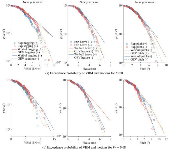Figure  18  Exceedance probability of peaks for the motions and VBM for the CT in the Draupner wave at Fn = 0 and Fn = 0.08

Download: Full-Size Img

for Fn = 0.08. For Fn = 0 and Fn = 0.08, the GEV model showed a better fit on the peak of motions and VBM, especially when Fn = 0, where significant deviations between the two distribution models were observed. Using the GEV distribution model, the most probable extreme values determined were 1.05×10⁶ kN·m in hogging and 1.15×10⁶ kN·m in sagging for VBM, 9.09° in positive and 8.21° in negative for the pitch and 6.15 m in positive and 6.90 m in negative for the heave. In the Peregrine breather solution (L_w/L_pp = 1.5) condition, the maximum values from the model tests were 1.129×10⁶ and − 1.529 7×10⁶ kN·m amidships, which are 7.5% and 33% higher than the extreme values from the Draupner wave tests. In the Peregrine breather solution (L_w/L_pp = 1.05) condition, the maximum value in hogging was 1.04×10⁶ kN·m, which is almost the same as the extreme value, and the peak value in sagging was − 1.43× 106 kN·m, which is slightly high.

The time series of the pressures and identified peaks at the bow for the CT in the Draupner wave at Fn = 0 and Fn = 0.08 are presented in Figure 19, and the exceedance probability of pressure peaks are illustrated in Figure 20. The maximum peaks were 0.946 2 and 3.23 bar, respectively for the two cases. Using the Weibull and GEV distribution, the most probable extreme values were 0.73 and 0.83 bar for Fn = 0, with the Weibull model showing a better performance. In the Peregrin breather solution with L_w/L_pp = 1.28 and L_w/L_pp = 1.5, the maximum peak pressures were 0.86 and 1.22 bar at sensor No. 2 (Figures 15(c) and 15(d)), and these values are 18% and 67% higher than the extreme values estimated using Weibull model in the Draupner wave condition. In regard to the case of Peregrin breather solution with L_w/L_pp = 1.05, the maximum peak was 0.78 bar, which is in good agreement with the extreme pressure (0.73 bar from Weibull). The findings indicate breather solutions as desirable alternatives to real work abnormal waves, in consideration of the slamming load issue.

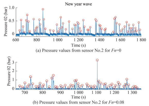Figure  19  Time series of the pressures and identified peaks at the bow for the CT in the Draupner wave at Fn = 0 and Fn = 0.08

Download: Full-Size Img

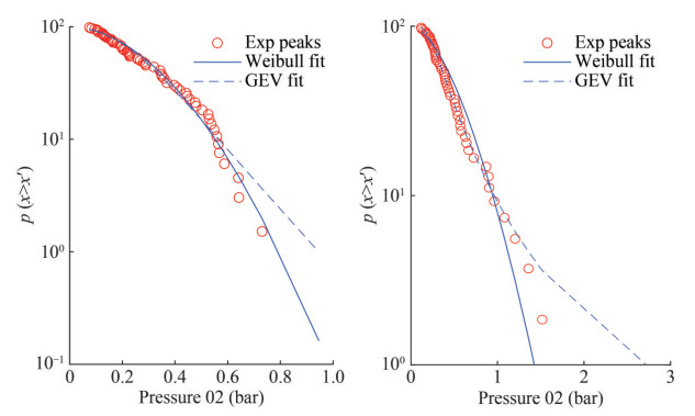Figure  20  Exceedance probability of pressure peaks at the bow for the CT in the Draupner wave at Fn = 0 and Fn = 0.08

Download: Full-Size Img

When Fn = 0.08, the most probable extreme values were 1.36 and 2.00 bar for Weibull and GEV distribution models, respectively. However, significant deviations were observed at the tails of the exceedance probability between the analytical distribution model and measured values. The Weibull model underestimated, and the other overestimated the extreme pressure peaks. In any case, the pressures increased with the increase in the forward speed of the model.

4   Conclusions

This study investigated the impact of extreme waves on the behavior of a CT. Experimental data from model tests in regular, irregular, and real-world extreme waves were analyzed in terms of the generated wave surface elevations, heave, pitch motions, vertical bending motions, slamming pressures, and green water. Some conclusions were drawn from the analysis:

1) Model tests conducted in high steep regular waves revealed that the asymmetry between hogging and sagging moments intensified as the wave steepness increased. Furthermore, green water on deck affected ship motions by inducing a counteracting moment.

2) Random uncertainty analysis of irregular wave test results indicated that uncertainties for motions and VBM were all below 1.8%, but they were considerably higher for slamming pressures (with a maximum of 10.5%). The forward speed of the ship did not result in substantially higher uncertainties on bow pressure but induced higher errors at the bow.

3) The GEV model provided better fits for the peaks of motions and VBM. Regarding pressure peaks, the Weibull model performed better for the bow, and the GEV model was more effective for the stern. Nevertheless, considerable deviations occurred at the tail of the exceedance probability curves for pressure peaks.

4) Statistical values of generated extreme waves, ship motions, VBM, and pressures with experiments were compared, and the results demonstrate that breather solutions are effective substitutes for real abnormal waves. The measured VBM attained the design vertical wave bending moment, with higher values observed for the Peregrine breather solution yielding. Regarding slamming pressures, peak values from breather solution extreme waves matched those from the Draupner extreme wave.

Breather solutions serve as powerful tools for the generation of tailored freak waves of critical wavelengths for wave/structure investigations on various ships. They are recommended to be applied in future research.

Appendix A   Details on ship model mass distribution

Appendix B   Details on pressure transducers

Table B1 presents the positions of pressure transducers on the hull and the X and Z-coordinates, that is, the corresponding Y-positions resulting from the according hull geometry. The positions are given in meters in the model scale, with the origin located at the aft perpendicular at the keel level (Figure 1).

For the model tests, the pressure transducer HKM375-1.7 Bar A from Kulite was installed. The signal amplifiers for the pressure transducers were custom-made, designed, and manufactured in-house. The motivation for the development of an in-house signal amplifier lay in the application area. The dynamic pressures were expected to be in an extremely small measurement range, and as a result, only a very low-noise amplifier can accurately detect the measured signals. Figure B1 presents time traces of two exemplary pressure transducers. The noise level is considerably lower compared with the measured values.

Nevertheless, experimental uncertainties were observed in the model tests, i. e., some of the pressure transducers showed unusual behavior during the model tests (cf. Figure B1(a)). This finding can be related to the different temperature compensation behavior of the sensors although all sensors should provide the same specifications, a circumstance that must be considered carefully for the interpretation of the measured results. The installed pressure transducers can be classified into three different types:

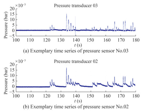B1  Time series of two pressure transducers with normal behavior

Download: Full-Size Img

• Regular behavior: no shifting pressure offset (cf. Figure B1(a)).

• Disputable behavior: a fast shifting offset related to the reference pressure during each wave impact (cf. Figure B1(b)) and a slow decay of the original reference pressure after each impact.

• Acceptable behavior: a fast shifting offset related to the reference pressure at the first wave impact, with the constant offset through the entire test run regarded as a new reference pressure level, i.e., no decay of the original reference pressure.

Appendix C   Details on investigated irregular sea states

Appendix D   Details on experimental uncertainty