
Influence of Elastic Modulus on the Dynamic Response of Polyester Mooring Under a Large Axial Stretch
https://doi.org/10.1007/s11804-024-00400-x
-
Abstract
Owing to the particularity of a polyester fiber material, the polyester mooring undergoes large axial tensile deformation over long-term use. Large axial tensile deformation significantly impacts the dynamic response of the mooring system. In addition, the degrees of large axial tension caused by different elastic moduli are also different, and the force on the mooring line is also different. Therefore, it is of great significance to study the influence of elastic modulus on the dynamic results of the mooring systems under large axial tension. Conventional numerical software fails to consider the axial tension deformation of the mooring. Based on the theory of slender rods, this paper derives the formula for large axial tension using the method of overall coordinates and overall slope coordinates and provides the calculation programs. Considering a polyester mooring system as an example, the calculation program and numerical software are used to calculate and compare the static and dynamic analyses to verify the reliability of the calculation program. To make the force change of the mooring obvious, the elastic moduli of three different orders of magnitude are compared and analyzed, and the dynamic response results after large axial tension are compared. This study concludes that the change in the elastic modulus of the polyester mooring changes the result of the vertex tension by generating an axial tension. The smaller the elastic modulus, the larger the forced oscillation motion amplitude of the top point of the mooring line, the more obvious the axial tension phenomenon, and the smaller the force on the top of the polyester mooring.-
Keywords:
- Large axial stretch ·
- Slender rod theory ·
- Polyester mooring ·
- Elastic modulus ·
- Dynamic response
Article Highlights● The motion equations for the large axial stretch of a polyester mooring were derived by combining the slender rod theory and shape function method.● The effect of large axial stretching on the motion response of a floating platform was considered.● The forces on the polyester mooring considering different elastic moduli and the operational response results with/without a large axial stretch with the same elastic modulus were compared. -
1 Introduction
Recently, with the evolution of ocean engineering in deep sea exploration, the materials used in the mooring lines have become a matter of concern. With the development of high-tech fibers, the performance of synthetic fiber materials fabricated from them has been greatly improved (Zhang and Xu, 2021). Nowadays, fiber materials with a tensile modulus of 10–30 GPa have found great attention, research efforts, and applications in marine engineering (Feng, 2016). However, the fiber cable creeps for a long duration, resulting in certain elongation, thereby reducing the stiffness (Li et al., 2021). The fiber cable has poor abrasion resistance and should be stored away from the fairlead and seabed and used in a suspended state (Pankina, 2021).
Fiber cables mainly involve polyester mooring, polypropylene, nylon, and other materials. Polyester mooring is widely used in the mooring systems of deepwater floating platforms due to its high strength, light weight, and good fatigue properties (Li et al., 2018). The research and application of polyester mooring in synthetic fibers are in their infancy (Wang et al., 2021). In terms of performance, the polyester cable has moderate tension under the same sea conditions, can suitably resist the effects of axial compression and creep, and has a large strength/weight ratio. Concurrently, polyester mooring has significant advantages in economy and reliability (Zhang et al., 2021). Polyester cable has nonlinear stiffness, which is highly complicated to study, and it changes with multiple factors such as the size of the loading force, duration, and number of cycles. Many scholars at home and abroad have conducted research on the mooring theory and the performance of polyester cable materials.
Liu et al. (2012) studied the nonlinear dynamic response of flexible mooring based on the slender rod theory and proved that the slender rod theory can obtain higher accuracy by using fewer elements. Ding et al. (2015) focused on the material nonlinearity of polyester cables and considered the coupling effect of Floating Production Storage and Offloading (FPSO). They used the dynamic time domain method to analyze the dynamic responses by using linear and nonlinear stiffness, respectively. The results demonstrated that compared with the polyester mooring with linear stiffness, the hull displacement obtained from the nonlinear stiffness polyester cable becomes larger, and the top tension value of the mooring line is extremely small. Mao (2019) used the static and dynamic stiffness simulation methods to understand the nonlinear characteristics of the axial stiffness of the polyester cable under different tension states of the deepwater semi-submersible platform mooring system. By calculating the force and movement of the semi-submersible platform mooring system and comparing the results with the numerical software, he found that the static–dynamic stiffness model to simulate the nonlinear stiffness of the semi-submersible platform mooring system's polyester cable performs reasonably and shows high calculation efficiency and accuracy.
Several studies have investigated the nonlinear stiffness characteristics of polyester mooring (Ding et al., 2015; Mao, 2019). However, because the polyester cable is a synthetic fiber material, after prolonged use, it stretches substantially, and the geometric shape of the polyester cable mooring changes, resulting in axial deformation (Segal et al., 2015). The axial stretch of the polyester cable could also have a significant impact on the overall mooring system. Welch and Tulin (1993) believed that the increase in the top mass would reduce the effective damping and increase the possibility of greater amplitude dynamic tension. They proposed a simple dynamic tension formula, which is approximated to the exact solution and includes the effect of axial strain.
Ma et al. (2015) used the Garrett slender rod model to describe the differential equation of the slender rod element through the shape function corresponding to the material points before and after the axial tensile deformation. They solved the combined effect of axial and bending deformations and considered a cantilever beam element model as an example to verify the convergence and accuracy of the rod element. Beltran et al. (2017) established a nonlinear mechanical model of the polyester cable and found that the friction effect (SLM) caused the deformation of the polyester cable to reduce the diameter of the polyester cable, thereby affecting the final result of static tension. They concluded that the influence of axial deformation of the nonlinear slender structure cannot be ignored.
As a slender structure, the process of solving the motion equation of the mooring line is extremely complex. Aamo and Fossen (2000) established the finite element model of the suspended cable in the water, calculated the hydrodynamic force on the cable using the Morison formula, ignored the additional mass of the cable, deduced the motion equation of the mooring line with fixed ends, and confirmed the existence and uniqueness of the overall solution of the system. Chen et al. (2001) established a model of the deep sea mooring system using a finite element method based on the slender rod theory and studied the dynamic interaction between the mooring system and the main body of the platform.
The polyester cable results in tension changes through axial deformation, thereby providing a horizontal restoring force to the platform. The accurate simulation of its nonlinear deformation characteristics is the key and basis for subsequent mooring system design. Based on the finite element model of a slender rod, this paper explores the geometric nonlinear relationship between axial stretch and bending deformations. The element model of the rod with large axial deformation is established, and the high accuracy characteristics of the calculation results of the slender rod model are retained.
2 Theory of large axial stretch
In marine engineering, the mooring line is a critical component with the characteristics of a slender geometric shape. The length–diameter ratio can reach above 1 000, which is prone to bending deformation, i.e., it has typical flexible characteristics (Gu et al., 2009; Zhang et al., 2012).
Slender rod theory is a numerical simulation theory of computation based on the vector mechanics method, which is established in the overall coordinate system to solve the large displacement, large rotation, and other large deformation problems of flexible slender rods. Compared with the traditional Euler–Bernoulli beam theory and the catenary theory, the slender rod theory is more accurate. (Shabana and Yakoub, 2001).
2.1 Force analysis of slender rod element
The advantage of the slender rod theory is that the motion control equation of the nonlinear flexible structure can be solved in the global coordinate system. The overall coordinates of the slender rod are shown in Figure 1. Among them, s is the arc length of the center of the unit; r is the position vector of the point on the centerline of the unit, which is a function of the arc length s and time t; (x, y, z) is the inertial coordinate; (eτ, en, eb) are the tangent, normal, and subnormal vectors of the arc length coordinates, respectively. A derivative relationship exists between (eτ, en, eb) and r, i.e., eτ = r′, en = r″, eb = r′ × r″, and |r′| = 1 (Cai et al., 2011).
 Figure 1 Slender rod element coordinate system
Assuming a unit δs on the space arc coordinates s. The force and torque on the unit are shown in Figure 2.
 Figure 2 Force and torque of the unit
According to the conservation law of momentum and angular momentum. The equilibrium equation of the unit is
$$\boldsymbol{F}^{\prime}+\boldsymbol{q}=\rho \ddot{\boldsymbol{r}}$$ (1) $$M^{\prime}+\boldsymbol{r}^{\prime} \times \boldsymbol{F}+\boldsymbol{m}=0$$ (2) where ρ is the mass matrix, F is the principal vector force of the section internal force at the arc length s; M is the principal vector moment of the section internal force at the arc length s. q and m are the distributed external force and distributed external moment on the unit.
2.2 Solving the differential equation of element rod motion
The unit balance equation adopts the overall coordinate and overall coordinate slope method. First, change the moment term M, including the bending moment term EIkeb and the torque term Heτ; EI is the bending stiffness, H is the torque, and K is the curvature and deflection at the arc length, then the M term can be written as
$$\boldsymbol{M}=E I \boldsymbol{k} \boldsymbol{e}_b+H \boldsymbol{e}_\tau$$ (3) According to the vector operation rule eb = eτ × en, the derivation of the bending moment and torque (Berzeri, 2000) is as follows:
$$\left(E I \boldsymbol{k e}_b\right)^{\prime}=\left(E I \boldsymbol{k} \boldsymbol{e}_\tau \times \boldsymbol{e}_n\right)^{\prime}=\boldsymbol{e}_\tau^{\prime} \times E I k \boldsymbol{e}_n+\boldsymbol{e}_\tau \times\left(E I \boldsymbol{k e}_n\right)^{\prime}$$ (4) $$\left(H \boldsymbol{e}_\tau\right)^{\prime}=H^{\prime} \boldsymbol{r}^{\prime}+H \boldsymbol{r}^{\prime \prime}$$ (5) $$\boldsymbol{e}_\tau^{\prime} \times E I \boldsymbol{k} \boldsymbol{e}_n=0$$ (6) $$e_\tau \times\left(E I \boldsymbol{k e}_n\right)^{\prime}=\boldsymbol{r}^{\prime} \times\left(E I \boldsymbol{r}^{\prime \prime}\right)^{\prime}$$ (7) M can finally be written as
$$\boldsymbol{M}^{\prime}=\boldsymbol{r}^{\prime} \times\left(E I \boldsymbol{r}^{\prime \prime}\right)^{\prime}+H^{\prime} \boldsymbol{r}^{\prime}+H \boldsymbol{r}^{\prime \prime}$$ (8) Generally, the torque in the slender structure is small; thus, the torque term can be ignored. Since this type of structure is completely immersed in the seawater, the waves and ocean currents become the environmental loads, and there is no distributed moment. Equation (2) can be written as
$$\boldsymbol{r}^{\prime} \times\left(E I \boldsymbol{r}^{\prime \prime}\right)^{\prime}+\boldsymbol{r}^{\prime} \times \boldsymbol{F}=0$$ (9) According to the cross-product theorem, if the cross-product value of two vectors is 0, the two vectors are parallel to each other, but the values of the vectors are not necessarily the same. Here, assuming that the difference between the two vectors is λ time, then
$$\left(E I \boldsymbol{r}^{\prime \prime}\right)^{\prime}+\boldsymbol{F}=\lambda \boldsymbol{r}^{\prime}$$ (10) $$\boldsymbol{F}=\lambda \boldsymbol{r}^{\prime}-\left(E I \boldsymbol{r}^{\prime \prime}\right)^{\prime}$$ (11) From this, the differential equation of motion of the element rod in the slender rod theory can be derived as follows:
$$\rho \ddot{\boldsymbol{r}}+\left(E I \boldsymbol{r}^{\prime \prime}\right)^{\prime \prime}-\left(\lambda \boldsymbol{r}^{\prime}\right)^{\prime}-\boldsymbol{q}=\mathbf{0}$$ (12) $$\boldsymbol{r}^{\prime} \cdot \boldsymbol{r}^{\prime}=1$$ (13) 2.3 Solving the differential equations of large axial stretch based on the shape function
When the axial tensile deformation is considered, strain presumably occurs per unit length, which is recorded as ε. The control Equation (13) of stretching is written as
$$\left|\boldsymbol{r}^{\prime}\right|=\left(\boldsymbol{r}^{\prime} \cdot \boldsymbol{r}^{\prime}\right)^{1 / 2}=1+\varepsilon$$ (14) $$\varepsilon=\frac{T}{E A}$$ (15) T is the tension of the top points. The variable λ in the moment balance equation is written as
$$\lambda=\left[\left(\frac{\boldsymbol{B} \boldsymbol{r}^{\prime \prime}}{\left|\boldsymbol{r}^{\prime}\right|^2}\right)^{\prime}+\boldsymbol{F}\right] \cdot \frac{\boldsymbol{r}^{\prime}}{\left|\boldsymbol{r}^{\prime}\right|}$$ (16) Inserting Equation (12) into integral processing:
$$\int_0^l\left[\rho \ddot{\boldsymbol{r}}+\left(E I \boldsymbol{r}^{\prime \prime}\right)^{\prime \prime}-\left(\lambda \boldsymbol{r}^{\prime}\right)^{\prime}-\boldsymbol{q}\right] a_i(s) \mathrm{d} s=0$$ (17) where ai is the original function in the substitution variable. The integral equation is simplified into an index form with a shape function as follows:
$$\begin{aligned} & \gamma_{i k m}(s) \boldsymbol{M}_{n j m} \ddot{\boldsymbol{u}}_{k j}+a_{i k m}(s) E I_m u_{k n} \\ = & \mu_{i m}(s) \boldsymbol{q}_{m n}+f_{i n}^{n b c}-\beta_{i k n} \lambda_m(t) u_{k n}\end{aligned}$$ (18) qmn is the drag force, which is calculated using the Morrison's formula:
$$\boldsymbol{q}_{m n}=\frac{1}{2} \rho_f D_f C_D \boldsymbol{V}_{m n}^N\left|\boldsymbol{V}_m^N\right|$$ (19) VmnN is the component value of normal velocity in all directions of the coordinate system. CD is the drag coefficient.
The constraint of stretching is
$$\beta_{i k m}(s) u_m u_{k n}-\tau_m(s)=0$$ (20) Among them, γikm (s), αikm (s), βikm, μim(s), τm(s) is the integral form of the original function, and finnbc is the resultant force of the unit. Assuming the axial large stretch, considering the presence of the node strain εm, the Equation (18) is changed to
$$\begin{aligned} & \gamma_{i k m}(s) \boldsymbol{M}_{n j m} \ddot{\boldsymbol{u}}_{k j}+\alpha_{i k m}(s) \frac{E I_m}{\left(1+\varepsilon_m\right)^4} u_{k n} \\ & =\mu_{i m}(s) \boldsymbol{q}_{m n}+f_{i n}^{n b c}-\frac{\beta_{i k m}(s)}{1+\varepsilon_m} \lambda_m(t) u_{k n}\end{aligned}$$ (21) The constraint control equation is changed to
$$\beta_{i k m}(s) u_m u_{k n}-\left(1+\varepsilon_w\right)^2 \eta_{w m}(s)=0$$ (22) Taking the element unknowns in Equation (21) and Equation (22) to obtain partial derivatives, the stiffness matrix form, including large axial stretch, can be formed (Ma, 2013):
$$\boldsymbol{K}=\left[\begin{array}{cc}\alpha_{i k m}(s) \frac{E I_m}{\left(1+\varepsilon_m\right)^4}+\frac{\beta_{i k m}(s)}{1+\varepsilon_m} \lambda_m & \frac{\beta_{i k m}(s)}{1+\varepsilon_m} u_{k n} \\ \beta_{i k m}(s) u_{i n} & -\frac{\eta_{l m}(s)}{E A_w^t}(1+\varepsilon)\end{array}\right]$$ (23) $$\begin{aligned} \boldsymbol{F}= & {\left[\begin{array}{c}\mu_{i m}(s) q_{m n}+f_{i n}^{n b c} \\ 0\end{array}\right] } \\ & -\left[\begin{array}{c}\alpha_{i k m}(s) \frac{E I_m}{\left(1+\varepsilon_m\right)^4} u_{k n}+\frac{\beta_{i k m}(s)}{1+\varepsilon_m} \lambda_m u_{k n} \\ \frac{1}{2} \beta_{i k m}(s) u_{i n} u_{k n}-\frac{1}{2} \eta_{w m}(s)\left(1+\varepsilon_w\right)^2\end{array}\right]\end{aligned}$$ (24) Then, the formulation (21) is changed to (Kim et al., 2004)
$$\boldsymbol{K} \cdot \boldsymbol{\varDelta}=\boldsymbol{F}$$ (25) Δ is
$$\boldsymbol{\varDelta}=\left[\begin{array}{l}u_{k n} \\ \lambda_m\end{array}\right]$$ (26) To this point, the calculation formula of the element rod considering the large axial stretch is deduced.
3 Validation of calculation program for polyester mooring
The calculation program of the polyester cable mooring considering the large axial stretch is written according to the theoretical formula of the element rod.
Considering the polyester mooring system as an example and comparing the results of the calculation program with those of the numerical software to verify the reliability of the results of the calculation program (Clukey et al., 2008). The water depth of the given sea area is 1 500 m, the composition of the polyester cable is anchor chain – polyester cable–anchor chain, wherein the upper and lower anchor chain parameters remain the same, the total length of the polyester cable is 1 530 m, and the horizontal distance between the fairlead and the anchor point is 700 m. The specific parameters of the mooring materials are shown in Table 1. The numerical calculation model by OrcaFlex is shown in Figure 3. Among them, the blue and brown lines represent the horizontal plane and the seabed, respectively.
Table 1 Parameters of polyester mooringAnchor chain Length (m) 100 Diameter (m) 0.1 E (N/m2) 1.5×10¹¹ Wet mass (kg/m3) 7 850 Polyester cable Length (m) 1 530 Diameter (m) 0.05 E (N/m2) 2×10¹⁰ Wet mass (kg/m3) 1 440  Figure 3 Numerical calculation model
The static iterative configuration of the polyester line is performed with the mooring parameters mentioned in Table 1, and the comparison of the theoretical and numerical simulation results of a static configuration of the chain–polyester–chain line are shown in Figure 4.
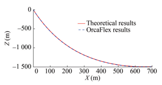 Figure 4 Comparison of theoretical and OrcaFlex results of a single polyester cable mooring configuration
The numerical software cannot accurately simulate the effect of large axial stretch on the dynamic response of the polyester cable mooring. Therefore, the effect of axial tension must not be considered in the results of program calculation and comparison with the numerical software.
The simple harmonic forced motion is applied to the top fairlead of the polyester mooring in the horizontal direction; the amplitudes are 5, 10, and 20 m; and the frequency ω is 0.6 rad/s. The stable section data from 100 to 200 s are extracted from the comparison results. The time history results and time–frequency conversion results of a single polyester line are shown in Figures 5, 7, and 9. The comparison results of the component forces in the X and Z directions under various amplitudes are shown in Figures 6, 8, and 10.
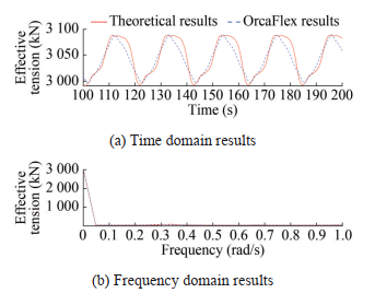 Figure 5 Comparison of theoretical and OrcaFlex results of effective tension (Amplitude is 5 m)
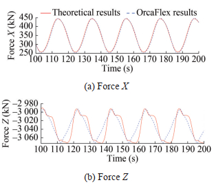 Figure 6 Comparison of theoretical and OrcaFlex results of the component force (Amplitude is 5 m)
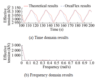 Figure 7 Comparison of theoretical and OrcaFlex results of effective tension (Amplitude is 10 m)
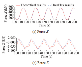 Figure 8 Comparison of theoretical and OrcaFlex results of component force (Amplitude is 10 m)
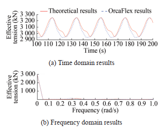 Figure 9 Comparison results of effective tension (Amplitude is 20 m)
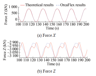 Figure 10 Comparison of theoretical and OrcaFlex results of component force (Amplitude is 20 m)
Figure 4 shows that the theoretically written polyester cable mooring calculation program is the same as the numerical software for the configuration of the mooring line, indicating that the polyester cable calculation program is accurate for the static iteration method of the mooring line parameters.
Figures 5–10 show that the comparison results of the dynamic response of the polyester cable calculation program and the numerical software, when the amplitude motion is applied, are the same, which verifies the accuracy of the program. Among them, the average error of the comparison results of the vertex effective tension, component force X, and component force Z at the respective amplitude of 5 m is 2%, 1.5%, and 1.7%. Moreover, the average error of the comparison results in other amplitudes is small, which is within the allowable range of error. Notably, the peak value of the comparison result of the component force Z in Figure 10 is different because although the length change caused by the large axial tension is not considered in the program setting, the resulting stress still affects the result. The difference between the numerical and theoretical calculation results during the intermediate process is caused by the difference between the calculation accuracy of the theory used in this article and that of the centralized mass method used by the OrcaFlex numerical simulation software.
4 Influence of the value of elastic modulus on the results of dynamic response
Equations (23) and (24) show that the large axial stretch is a process wherein the strain changes with the stress, and the degree of change is related to the value of the elastic modulus.
The third chapter discusses that the calculation program based on the theory is consistent with the comparison results of the numerical calculation software OrcaFlex. To reflect the influence of large axial tension more intuitively, it is necessary to compare the theoretical results of large axial tension with the results of the numerical software.
The modulus of elasticity can be regarded as an index to measure the degree of difficulty in the elastic deformation of a material. The greater the value, the greater the stress causing the material to undergo a certain elastic deformation (Tahar and Kim, 2008).
To reduce the interference of other variables on the results, a single mooring making the length of the anchor chain segment and the polyester mooring segment close is selected as the research object, and different levels of elastic modulus are selected in the polyester cable segment for calculation. Further, the accuracy of the polyester cable calculation program based on the slender rod theory is verified.
The water depth of the given sea area is 420 m, and the mooring line is composed of an anchor chain–polyester cable–anchor chain. The total length of the mooring line is 1 300 m, and the horizontal distance between the fairlead and the anchor point is 1 170 m. The specific material parameters are shown in Table 2.
Table 2 Parameters of the polyester mooring considering the change in the elastic modulusAnchor chain Length (m) 400 Diameter (m) 0.286 E (N/m2) 2.98×10¹¹ Wet ness (kg/m3) 7 850 Polyester cable Length (m) 500 Diameter (m) 0.15 E (N/m2) 2×10⁸/2×109/2×1010 Wet ness (kg/m3) 1 440 Since it is necessary to compare the influence of the elastic modulus of the polyester cable segment on the dynamic response results, the elastic modulus must agree with reality (1×10⁸–1×10¹¹). A simple harmonic forced motion in the horizontal direction is applied to the fair lead of the polyester cable. The amplitude is 5, 10, and 20 m, the frequency ω is 0.3 rad/s. The axial stretching amount is different under different amplitude motions. When the motion amplitude is 5 m, the mooring elongation of the polyester mooring considering axial stretching is 3.2 m longer than that without a stretch; when the amplitude is 10 m, this value is 6.56 m; when the amplitude is 20 m, this value is 14.67 m. Although there is a certain amount of axial stretch, it changes little compared with the whole mooring line. The data of the stable section in the calculation results are extracted, and the comparison time history results of the apex tension of the elastic modulus of the polyester cable are obtained at different levels, as shown in Figures 11‒13.
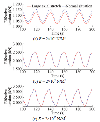 Figure 11 Comparison results of effective tension under different elastic modulus (Amplitude is 5 m)
 Figure 12 Comparison results of the effective tension under different elastic moduli (Amplitude is 10 m)
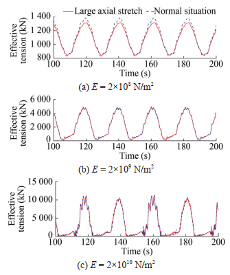 Figure 13 Comparison results of effective tension underdifferent elastic modulus (Amplitude is 20 m)
The comparison results of the dynamic response of different elastic moduli show that when the elastic modulus is 2×10⁸ N/m2 (Figure 11) (Amplitude is 5 m), whether the effective tension of large axial stretch is considered or not, the maximum difference at the peak is 82.3 kN, and the maximum difference in Figure 12 (Amplitude is 10 m) is 92.1 kN. In Figure 13 (Amplitude is 20 m), the maximum difference is 101.7 kN. When the moduli of elasticity are 2×10⁹ and 2×10¹⁰ N/m2, almost no difference is observed with or without considering the dynamic response results of the large axial stretch. Alternatively, when the bending stiffness and tension consider the large axial tension caused by strain transformation, the periodic peak of motion will get smaller stress response results compared with the normal case. This is also consistent with the conclusion of Equations (21) and (22). As the stress ε increases, K would decrease and affect the size on the right side of Equation (25). Irrespective of the amplitude of motion, when the elastic modulus is 2×10⁸ N/m2, a great difference exists between the effective tension under consideration of large axial tension and that under normal conditions, with the latter being greater than the former. In other words, when the magnitude of the elastic modulus is relatively small (2×10⁸ N/m2 in this paper), the effective tension at the top of the polyester cable will decrease under large axial tension.
5 Conclusions
As described in this paper, polyester is prone to tensile deformation. Conventional numerical software does not consider the impact of large axial tension on the response results in the mooring of a polyester cable. Owing to the long-term use of the mooring system, the polyester cable section could have a large axial stretch, which can considerably impact the dynamic response of the floating platform. The results and conclusions of this paper are as follows.
Based on the slender rod theory, combined with the shape function, the calculation equation of the large axial stretch was derived. Comparing the written calculation program with the results of the numerical software has proven the correctness and reliability of the deduced equation and written calculation program.
Considering the change in the strain magnitude, the dynamic response results of large axial deformation were compared under different elastic moduli. The smaller the modulus of elasticity, the greater the difference between the dynamic response results of a large axial stretch.
Under the same modulus of elasticity, as the amplitude of the given simple harmonic motion increases, the difference between the dynamic response results with and without considering the axial stretch increases.
Polyester mooring will inevitably have a large axial stretch. This paper concludes that increasing the elastic modulus of a polyester cable can effectively reduce the influence of a large axial stretch.
Competing interest Liping Sun is an editorial board member for the Journal of Marine Science and Application and was not involved in the editorial review, or the decision to publish this article. All authors declare that there are no other competing interests. -
Figure 1 Slender rod element coordinate system
Figure 2 Force and torque of the unit
Figure 3 Numerical calculation model
Figure 4 Comparison of theoretical and OrcaFlex results of a single polyester cable mooring configuration
Figure 5 Comparison of theoretical and OrcaFlex results of effective tension (Amplitude is 5 m)
Figure 6 Comparison of theoretical and OrcaFlex results of the component force (Amplitude is 5 m)
Figure 7 Comparison of theoretical and OrcaFlex results of effective tension (Amplitude is 10 m)
Figure 8 Comparison of theoretical and OrcaFlex results of component force (Amplitude is 10 m)
Figure 9 Comparison results of effective tension (Amplitude is 20 m)
Figure 10 Comparison of theoretical and OrcaFlex results of component force (Amplitude is 20 m)
Figure 11 Comparison results of effective tension under different elastic modulus (Amplitude is 5 m)
Figure 12 Comparison results of the effective tension under different elastic moduli (Amplitude is 10 m)
Figure 13 Comparison results of effective tension underdifferent elastic modulus (Amplitude is 20 m)
Table 1 Parameters of polyester mooring
Anchor chain Length (m) 100 Diameter (m) 0.1 E (N/m2) 1.5×10¹¹ Wet mass (kg/m3) 7 850 Polyester cable Length (m) 1 530 Diameter (m) 0.05 E (N/m2) 2×10¹⁰ Wet mass (kg/m3) 1 440 Table 2 Parameters of the polyester mooring considering the change in the elastic modulus
Anchor chain Length (m) 400 Diameter (m) 0.286 E (N/m2) 2.98×10¹¹ Wet ness (kg/m3) 7 850 Polyester cable Length (m) 500 Diameter (m) 0.15 E (N/m2) 2×10⁸/2×109/2×1010 Wet ness (kg/m3) 1 440 -
Aamo OM, Fossen TI (2000) Finite element modeling of mooring lines. Mathematics and Computers in Simulation 5(53): 415–422. DOI: 10.1016/S0378-4754(00)00235-4 Beltran JF, Ramirez N, Williamson E (2017) Simplified analysis of the influence of strain localization and asymmetric damage distribution on static damaged polyester rope behavior. Ocean Engineering 145: 14–17. DOI: 10.1016/J.OCEANENG.2017.09.006 Berzeri M, Shabana AA (2000) Development of simple models for the elastic forces in the absolute nodal co-ordinate formulation. Journal of Sound and Vibration 235(4): 539–565 https://doi.org/10.1006/jsvi.1999.2935 Cai Fengchun, Zang Fenggang, Ye Xianhui, Huang Qian (2011) Analysis of nonlinear dynamic behavior of pipe conveying fluid based on absolute nodal coordinate formulation. Journal of Vibration and Shock 30(6): 143–146, 157. DOI: 10.13465/j.cnki.jvs.2011.06.032 Chen Xiaohong, Zhang Jun, Ma Wei (2001) On dynamic coupling effects between a spar and its mooring lines. Ocean Engineering 28(7): 863–887. DOI: 10.1016/S0029-8018(00)00026-3 Clukey E, Jacob P, Sharma PP (2008) Investigation of riser seafloor interaction using explicit finite element methods. Offshore Technology Conference, Houston, OTC-19432-MS. DOI: 10.4043/19432-MS Ding Haijian, Qian Jiayu, Tao Jun (2015) Influence of nonlinear stiffness on deep mooring system. Ship Engineering 37(4): 84–97. DOI: 10.13788/j.cnki.cbgc.2015.04.084 Feng Limei (2016) Usage of polyester rope in deepwater mooring system. Ocean Engineering Equipment and Technology 3(5): 315–319 Gu Chujiang (2009) Study on lectotype of tidal current power platform and mooring system design. PhD thesis, Harbin Engineering University, Harbin Kim N, Jeon SS, Kim MY (2004) Nonlinear finite element analysis of ocean cables. China Ocean Engineering 18(4): 537–550 Li Da, Bai Xueping, Wang Wenxiang (2018) Research on key technologies for design of deep water FPSO single point mooring system in South China Sea. China Offshore Oil and Gas 30(4): 196–202. DOI: 10.11935/j.issn.1673-1506.2018.04.025 Li Hangyu, Li Maoben, Li Yanxi (2021) Review of fiber mooring polyester ropes for deep sea floating structures. International Core Journal of Engineering 7(5): 122–127. DOI: 10.6919/ICJE.202105_7(5).0045 Liu Wenxi, Zhang Weikang, Ren Huilong (2012) Calculation of nonlinear dynamic response of mooring lines. Shipbuilding of China 53(2): 39–50 Ma Gang (2013) Nonlinear dynamic response analysis of slender rods in deepwater. PhD thesis, Harbin Engineering University, Harbin Ma Gang, Sun Liping, Ai Shangmao (2015) A nonlinear mechanical model for extensible slender rod. Applied Mathematics and Mechanics 36(4): 371–377. DOI: 10.3879/j.issn.1000-0887.2015.04.004 Mao Chengliang (2019) Nonlinear stiffness simulation analysis of polyester ropein deep ocean semi-ubmersible platform. Ship Engineering 48(1): 112–116. DOI: 10.3963/j.issn.1671-7953.2019.01.026 Pankina SI, Umanskaya LA, Lyutikova M, Malakhov SO, Syusyuka E (2021) Analysis of the accident consequences at the remote mooring facilities of the Caspian Pipeline Consortium. IOP Conference Series: Earth and Environmental Science 872(1): 012025. DOI: 10.1088/1755-1315/872/1/012025 Segal EM, Rhode-Barbarigos L, Adriaenssens S, Coelho RDF (2015) Multi-objective optimization of polyester-rope and steel-rope suspended footbridges. Engineering Structures 56(6): 99–105. DOI: 10.1016/j.engstruct.2015.05.024 Shabana AA, Yakoub RY (2001) Three-dimensional absolute nodal coordinate formulation for beam elements: theory. Journal of Mechanical Design 123(4): 606–613 https://doi.org/10.1115/1.1410100 Tahar A, Kim MH (2008) Coupled-dynamic analysis of floating structures with polyester mooring lines. Ocean Engineering 35(17): 1676–1685. DOI: 10.1016/j.oceaneng.2008.09.004 Wang Zhifeng, Du Chunshui, Gao Chao (2021) Deepwater polyester cable mooring technology and application. Nem Technology & Products of China 30(5): 39–42. DOI: 10.13612/j.cnki.cntp.2021.05.012 Welch SM, Tulin MP (1993) Axial cable stretching due to strumming and possibility for resonance. Proceedings of the Third International Offshore and Polar Engineering Conference, 364–369 Zhang Ding, Xu Yangguang (2021) Fluence of different combinations of mooring line on characteristics of FLNG single point mooring system. China Offshore Oil and Gas 33(5): 175–181. DOI: 10.11935/j.issn.1673-1506.2021.05.022 Zhang Ruoyu, Tang Yougang, Song Jizhe, Liu Liqin (2012) Analysis of dynamic tension nonlinear characteristics for mooring system in the deep water. Journal of Ship Mechanics 16(7): 804–811 Zhang Yang, Chai Zhuang, Wang Wenhua (2021) Dynamic stiffness characteristic of deep-sea mooring cable. Ship Engineering 43(2): 149–155. DOI: 10.13788/j.cnki.cbgc.2021.02.03
