1   Introduction

Seakeeping codes in the frequency domain have been developed based on the potential flow theory and diverse methodologies to solve the motion equations of advancing ships over a range of incident waves. In the potential flow hypothesis, inertia potential, diffraction potential and radiation potential are identified in the frequency domain to obtain the velocity potential fields of three-dimensional NeumannKelvin formulation over different ranges of validity. For instance, the slender body assumption has been imposed into the computations for the strip theory to determine the hydrodynamic coefficients of advancing ships over a range of wave frequencies (Salvesen et al., 1970). Though the added mass and damping coefficient of the ship would be calculated by integrating the hydrodynamic coefficients of each cross-section at the encounter frequency along the ship length, the longitudinal component of normal vector on ship form has been neglected in the strip theory. Therefore, to extend the range of validity of the frequency domain algorithm, three-dimensional boundary integral equations have been implemented into the algorithm by such as Bingham and Korsmeyer (1994), Nakos et al. (1991), Newman (1979) and Xia et al. (1998).

Different review papers provided an overview of the codes available (Hirdaris et al., 2014; Temarel et al., 2016; Parunov et al., 2022a; 2022b) and several benchmark studies have been performed over the years to assess the skill of the various codes available, both based on the strip theory and the 3D boundary element formulations, such as those presented by Schellin et al. (1996), Bunnik et al. (2010), Kim and Kim (2016) and Parunov et al. (2020, 2022a). In general, these studies showed that the strip theory codes do not provide the same results as the panel codes. The benchmark studies have been a good instrument for the modelling of the uncertainty in the predictions, an effort that has also been made throughout the years (Guedes Soares, 1991; Kim and Hermansky, 2014; Parunov et al., 2022b) and applied to many practical problems (Ćatipović et al., 2019; Gaeta et al., 2020).

Several frequency domain seakeeping codes have been commercialized such as WAMIT, WASIM, HydroSTAR, ANSYS-AQWA and MAXSURF which have been largely used for different applications such as the design of floating structures (Wang and Lu, 2011; Belibassakis et al., 2009). Some of these codes have come up with limitations, as some of them are valid only for a low range of advancing speeds (Froude number < 0.2), which is good to be used for offshore structures but restricts the range of applicability to ships with forward speeds.

The frequency domain algorithms impose two underlying assumptions including linearized free surface boundary conditions and the linear body boundary condition into the solution. To implement the nonlinear formulation into the boundary value problem, the Dawson method has been largely applied on the free surface (Abbasnia et al., 2015; Celebi et al., 1998). Taylor's series has been used to discretize the nonhomogeneous nonlinear terms of the exact free surface boundary conditions and the complexity of deriving high-order truncated terms discourages the formulation for further applications.

On the other hand, the nonlinear potential codes, which have been developed (Tang et al., 2021; 2023; Liu, 2019; Li and Long, 2020; Mei et al., 2020), are very demanding computationally and thus they are not cost-effective to be adopted in the ship's design process. Indeed, the time-domain nonlinear potential codes have come with a massive burden of computation and robust numerical instabilities although some codes such as GLRankine (Söding and Bertram, 2009) and SIS (Söding, 2020) proved to be rather reliable and accurate. A compromise solution adopted by several authors is to use formulations in the time domain based on the strip theory, several of which are compared by Watanabe and Guedes Soares (1999).

A retrospective analysis of contributions to the seakeeping hydrodynamics indicates that while the strip method proved to be adequate for slender ships, there is the necessity to predict motions and wave loads on floating structures of quite different configurations for which the application of the strip theory is inadequate. This stimulated the development of 3D codes since the late 70 s and 80 s which was already possible based on the available computing resources.

It must be said that despite the better inherent accuracy of time-domain nonlinear codes, linear frequency-domain codes proved to be significantly faster while sufficiently accurate for many applications. The already mentioned commercial program WAMIT is probably the most widely known example of such software. However, while commercial programs are suitable for practical engineering computations, research applications often make access to the source code and full command of the algorithm highly desirable. That is why several in-house programs were developed at various institutions and are typically preferred there to their commercial analogues. As an example of such in-house code, the frequency-domain linear seakeeping program DELFRAC was developed in Fortran 77 in the 80 s and 90 s at the Delft University of Technology (Dmitrieva, 1994).

The code SEAKIST developed within the present study is in many respects similar to DELFRAC but quite independent of it. Preliminary advances in the code's development are described in Abbasnia et al. (2021; 2022) while the present contribution exposes some further developments and validation. Unlike DELFRAC, this code is written in C++ language with substantial use of the object-oriented paradigm. At first glance, this feature may seem secondary and not essential, but the authors' experience proves that an object-oriented structure makes the code more transparent and much more convenient for maintenance and modifications which are constantly required in exploratory studies. From this viewpoint, this program presents some novelty.

Back some years, a double-body potential flow panel code has been developed for predicting interaction forces for ships manoeuvring in close proximity (Sutulo et al., 2012). The code later named HYDINTER (Sutulo and Guedes Soares, 2016) was based on the Hess & Smith method and was primarily programmed in Fortran 90 language but later translated into C++ to facilitate its merging with a manoeuvring simulation code.

To transform the double body interaction code into a seakeeping one, it was necessary to properly account for the free-surface boundary condition. This is achieved by adding an appropriate regular part to the source potential, and modifying the source Green function in such a way that the frequency-dependent free-surface boundary condition is satisfied. Although analytical solutions for the potential of a pulsing source beneath the free surface had been obtained many years ago, its efficient and accurate computation presented a non-trivial numerical problem. Within the WAMIT package, this problem is solved by the Fortran 77 subroutine FGREEN which is also being distributed by the developers on a commercial basis. That subroutine on the level of the source code was purchased and used "as is" by the developers of the program DELFRAC and had also been purchased by IST some time ago. That made its embedment into the SEAKIST code possible but, as long as the authors desired to avoid complex pieces written in different languages, the Fortran code was translated into C++ which resulted in the C++ function named FinGreen (Abbasnia et al., 2021).

Further development was aimed at solving the diffraction problem for slowly advancing ships through a range of wave frequencies in arbitrary heading angles. The code was verified for vertical motions with sets of experimental measurements in a container ship by Abbasnia et al. (2022). The present version of the SEAKIST represents a further step that yields the determination of the vertical shear force and the vertical bending moment for a stationary as well as for an advancing ship and provides validation of the computation results against experimental results of a containership and an LNG carrier.

Section 2 of the present paper presents a brief exposure of a rather standard theory lying behind the SEAKIST code and Section 3 briefly presents some details of the numerical algorithm. All numerical results related to the grid convergence study, verification and validation of the code are presented in Section 4 while the last section contains the conclusions.

2   Computational model development

The assumptions for the linear seakeeping theory are applied. The flow can be completely described by the velocity potential satisfying the Laplace equation, the linearized freesurface boundary condition and the non-penetration condition on the oscillating hull assumed to be fixed in the equilibrium position. To take advantage of the frequency domain calculation for the advancing ships in waves, three coordinate systems are assumed including the global fixed coordinates system, the hydrodynamic coordinates system and the local coordinates system. The hydrodynamic coordinates system is placed on the advancing ships to measure the oscillations of ships. Therefore, the origin of the hydrodynamic coordinates system is the centre of rotation of ships. The local coordinates system sticks to the ship hulls to calculate the potential flow over the wetted surface.

In the frame of the global coordinates systems, the total velocity potential function for advancing ships in waves comprises the uniform flow in the opposite of the ship heading, the incident wave velocity potential and the disturbance potential function induced by the presence of the floating body. The presence of the ship provokes disturbance in the uniform flow potential which causes wave-making resistance, and it disturbs the wave regimes which leads to the diffraction potential function and the radiation potential function. Hence, to solve the wave interaction with ships, the hydrodynamic coordinates system is deployed to solve the diffraction and radiation potential functions. In the following exposure, the encounter frequency ω_e will be used and is defined as

where β represents the relative angle of the incident wave to the ship's heading direction. V_s is the ship's speed, ω is the absolute frequency of the incident wave in the fixed global coordinate system linked with the wave number K through the linear dispersion relation. Eventually, the total velocity potential induced by the presence of advancing ships in waves is defined in the moving hydrodynamic coordinates system (Oxyz) shown in Figure 1, as

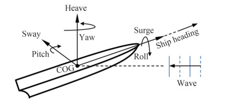Figure  1  The schematic scheme of the coordinate system of the wavebody problem

Download: Full-Size Img

The origin of the moving coordinates frame is allocated on the still water and the z-axis is directed upward. The wave amplitude is denoted by ζ and ϕ_D is the diffraction potential which is composed of the inertia and scattering components. The amplitudes of the ship responses are denoted by X_j in six-degree of freedom (j = 1, 2, …, 6) and the induced velocity potential due to unit oscillation at each mode of motion is defined as the radiation potential ϕ_j.

Applying the method of hydrodynamic singularities, it is possible to reduce the radiation-diffraction problem to the Fredholm integral equation:

where Γ is the computational boundary (the ship hull surface) and P(x, y, z) represents the field point and q (x′, y′, z′) is the source point which is distributed over the computational boundary. The strength σ () of the distributed source points. n = (n₁, n₂, n₃) is the unit normal vector on the computational boundary and it is directed outward of the fluid. The given boundary condition is denoted by ψ (). The pulsating free surface Green's function G () is given as

and $ r=|\boldsymbol{P}-\boldsymbol{q}|, \bar{r}=\left|\boldsymbol{P}-\boldsymbol{q}^{\prime}\right|$ in which $ \boldsymbol{q}^{\prime}=\left(x^{\prime}, y^{\prime}, -z^{\prime}\right)$. $\tilde{G} $() is the regular part of the Green function which stands for the free-surface effects on the induced potential flow due to the source pulsating in the frequency ω_e. The Green function satisfies the coupled linear free surface boundary condition and the radiation condition at infinity. Implementation of corresponding boundary conditions to radiation and diffraction velocity potential will result in the corresponding source densities. The hull boundary condition is:

where

Sweeping the field point over the locations of distributed source points for either the radiation potential boundary condition or the diffraction potential boundary condition gives off a system of equations and the strength of source points for each mode of radiation potential as well as for the diffraction potential is obtained. Eventually, integrating the strengthened source points leads to the velocity potential components. For instance, the radiation potential for each mode of motion at an arbitrary field point is calculated as

The radiation potential function is taken into account of hydrodynamic coefficients for each mode of motion and a boundary integral equation is given as

in which ρ is the water density. Introducing the added mass coefficients A^kj and the damping coefficient D^kj this function can be re-written as

Then, the set of linear algebraic equations for the complex amplitudes of the ship motions takes the form:

where M^kj and C^kj represents the global mass matrix and the restoring coefficient respectively which are driven by the hydrostatic characteristics of the ship's hulls. F_k stands for the exciting loads driven by the incident wave and the diffraction potential function is in the charge of scattered incident wave potential. By taking advantage of the Haskind– Newman relation, the diffraction potential does not need to obtain and the exciting loads coefficient is calculated as

In the left-hand side of the equation, the first term of the integrand takes responsibility for the Froude–Krylov loads and the second term corresponds to the diffraction potential. Eventually, the amplitude of the ship's motions would be determined from Equation (10). Furthermore, the general form of vertical shear force at any longitudinal location of the ship is obtained through the quasi-static equilibrium equation between the inertia forces and the resultant hydrodynamic vertical force acting on the fractional wetted surface forward of that longitudinal location as

where ℓ is the length of the fractional wetted surface and η is the wave profile; B () is the maximum ship breadth alongside the water plane and ρ is the water density and g represents the gravitational acceleration. The wave elevation is not taken into account commonly in the linear solution. Indeed, the linear assumption of the small amplitude of wave elevation rather than the ship draft and the wavelength leads to the negligence of wave elevation in calculating the restoring force and in updating the wetted surface. $\tilde{F}_3 $ and $\tilde{R}_3 $ are the fractions of the exciting force and the radiation force at the heave mode of motion. $\tilde{F}_3 $ is computed using Equation (11) and $\tilde{R}_3 $ is calculated as

where $ \tilde{f}_{3 k}$ is computed through the body integral of Equation (9) over the fractional wetted surface. Correspondingly, the vertical bending moment would be obtained through the longitudinal integration of the shear force components along the length ℓ.

3   Numerical algorithm and implemetation

The interaction of the underlying functions in the SEAKIST is sketched through the flow chart in Figure 2 in which the sequence of the development is pointed out. The HYDINTER function is in charge of solving the double-body boundary integral equation and the quadrilateral flat panel is devoted to the numerical discretization of Equation (3), written as

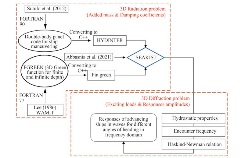Figure  2  The SEAKIST breakdown flowchart

Download: Full-Size Img

where δ_m′m is the Kronecker Delta function and $ \rlap{—} N$ denotes the number of panels on the wetted surface of the ship's hull. Spatial numerical integration is carried out in line with the constant increment which leads to defining the term of

The source points are allocated at the centroid of each panel and the $\tilde{G}_n^{(-)} $ is given through the FinGreen function. Fusing the FinGreen into the HYDINTER made the SEAKIST applicable for solving the radiation problem for a stationary ship hull. The resulting algebraic system of equations is always well-conditioned and the direct Gauss– Jordan method is applied to solving it. Then, the radiation potential function would be achieved by replicating the given strength of source points for each mode of motion in Equation (7) as given

Afterwards, SEAKIST was extended by a set of auxiliary functions to deal with the wave interaction with advancing ship hulls. Hydrostatic properties such as the centre of floatation, and exciting hydrodynamic loads are perquisites to solving the motion equation of ship hulls (Equation (10)). Hydrostatic properties are required to fulfil the mass matrix and the restoring matrix whereas Equation (11) is implemented to calculate the wave loads on the right-hand side of Equation (10).

The ship advance is considered through the encounter frequency and the solution of the radiation potential problem for each mode of motion is substituted into Equation (11) to achieve the hydrodynamic load at the corresponding mode of motion, as written as

4   Code verification and numerical results

4.1   LNG ship

The responses of an LNG carrier in a range of frequencies are used for additional verification of the SEAKIST solver. The experimental and numerical data of the LNG response were presented by Zhang et al. (2022) and Klein et al. (2023). The geometrical characteristics of the LNG ship are listed in Table 1 and the cross-sectional body is sketched in Figure 3. The vertical side wall for the part above the mean water line is postulated.

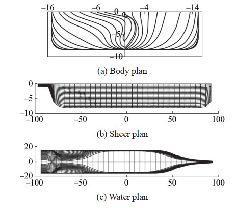Figure  3  The sketch of heading angles

Download: Full-Size Img

Quadrilateral panels are used to describe the ship hull which can be used to calculate the hydrostatic characteristics of the ship as well as to discretize the boundary integral equation.

A convergence test is carried out to examine the mesh dependency of the code for the panel number in Table 2.

The relative variation R of the values of four estimated parameters including the heave added mass and damping coefficients in heave and pitch are given by

where P_j is the parameter's value corresponding to the variant j in Table 2. It can be concluded from Table 2 that a definite internal convergence is observed for the variants from 1 to 4, and further augmentation of the number of panels shows signs of divergence. The panelisation variant with 1 152 panels (Figure 4) is used in further computations.

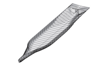Figure  4  The discretized ship hull

Download: Full-Size Img

The limitation of the panel method is the size of the panels which makes the condition of the coefficient matrix near singular and leads a significant difference for the finest meshes. This issue is raised from the Kernel terms (related to 1/r terms) of the Green function and the yielded near singular coefficient matrix makes the solution of the system of equations diverged.

The ship is exposed to the range of frequencies in zerospeed head-wave and the response amplitude operator (RAO) for heave, pitch motion, the vertical shear force (VSF) and the vertical bnding moment (VBM) at amidship are compared with the experimental data as shown in Figure 5. Computations are performed for the unity wave amplitude and for 90 frequencies whose range complies with the experimental data. The translational motion amplitude is normalized by the wave amplitude whereas the wave slope amplitude Kζ is used to normalize the rotational motion amplitude. Hence, X stands for the normalized surge motion, Y represents the normalized heave motion and Ω is the non-dimensional pitch motion. The non-dimensional amplitude of the VSF is defined as $\mathrm{VSF}=F_v / \rho g L_{\mathrm{pp}} B \zeta $ where F_v stands for the amplitude of the shear force at the midship section. Analogously, the VBM is normalized by $\mathrm{VBM}=\rho g L_{\mathrm{pp}}^2 B \zeta $ where B is the maximum breath of the ship and L_pp is the length between ships perpendiculars.

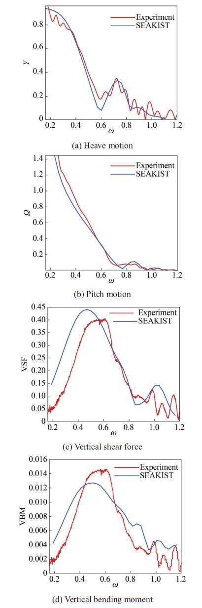Figure  5  Comparison of LNG response with the experiment (Zhang et al., 2022) over a range of angular frequencies

Download: Full-Size Img

The motion responses (Figures 5(a), 5(b)) are consistent with the experimental data confirming the earlier good comparisons of the motions of the S-175 container ship (Abbasnia et al., 2022). The validation of the loads, done here for the first time, shows that the maximum values of the VSF and VBM are close to the experimental values, the discrepancies between the VSF and the VBM and the experiments become larger while the wave frequency is decreasing. For the wave frequency ω ≃ 0.55 rad/s at which the significant hogging and sagging are expected, the SEAKIST results agree reasonably well with the experimental data for motion response as well the vertical loads. Larger disagreements of VSF and VBM than the RAO results might be triggered by numerical errors in calculations of spatial integration of hydrodynamic pressure on the wetted surface. Hence the error of potential flow solution is accumulated in the computation of the VSF and the VBM and moreover the incompliance of the mass distribution along the ship between the numerical and the experimental data makes inevitable additional error. To examine the functionality of SEAKIST once the LNG ships imposed to the range of wave frequencies in different angles (Figure 6), the response of the LNG carrier for five heading angles is shown in Figure 7. For ω < 0.55 rad/s, the VSF and the VBM amplitudes for heading angles 0° and 180° are consistent while the difference is becoming greater as the wave frequency increases.

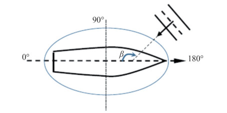Figure  6  The sketch of heading angles

Download: Full-Size Img

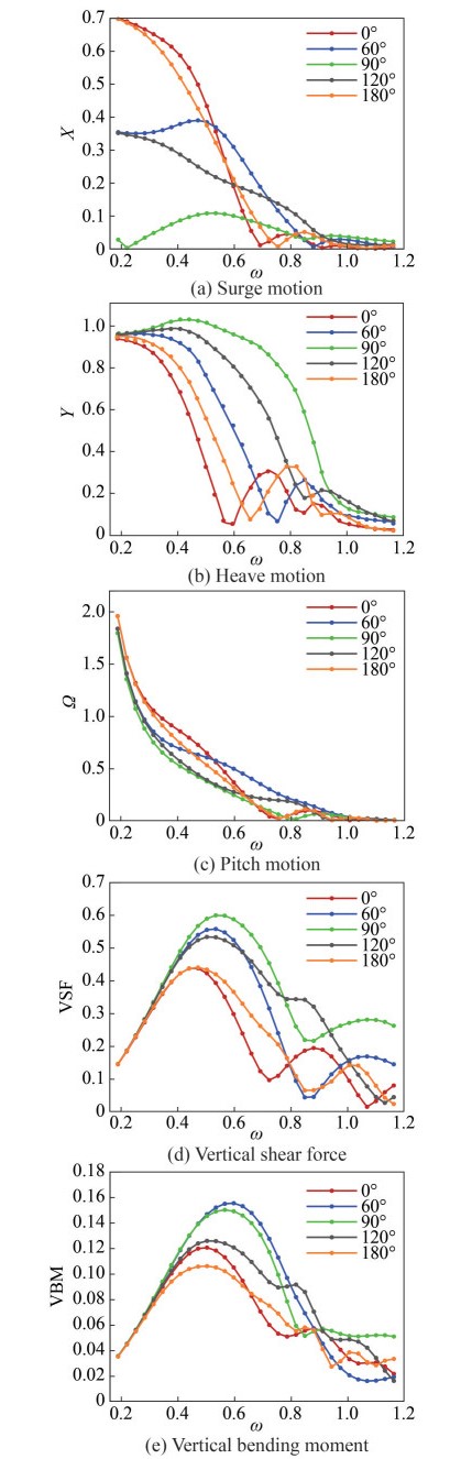Figure  7  The SEAKIST results for the LNG carrier in different angles of heading

Download: Full-Size Img

The same trend is observed on the VSF for the heading angles 60° and 120° over ω > 0.55 rad/s. Meanwhile, the difference between the VBM for the heading angles 60° and 120° is substantially larger than the VSF which might be triggered by the numerical integration of the shear force components along the ship length.

It implies that the effect of longitudinal asymmetry of the ship hull on the vertical loads is vanishing for the longer waves. Moreover, the longitudinal asymmetry effect on the heave motion for the oblique wave is more predominant than the head sea as well as the following sea. Analogously, the pitch motion comparison manifests the same trend. As expected, the surge motion amplitude for 90° is infinitesimal for the long waves, whereas the surge motion is amplifying for the shorter waves 0.3 < ω < 0.8 which are induced by the ship's longitudinal asymmetry. Moreover, the surge motion is reasonably tracking an attenuation trend for the heading angles 0° and 180° while the wave frequency is increasing.

4.2   S-175 containership

To assess the performance of SEAKIST for advancing ship hulls in different heading angles over a range of frequencies, the motion responses of the S-175 container ship were presented by Abbasnia et al. (2022) and the numerical results were compared to the experimental data reported in ITTC (1983). In this paper, the same case study is replicated and extended to calculate the VSF and the VBM at the amidships and the results are compared with the experimental data in Figure 8 for the Froude number $ F n=V_s / \sqrt{g L_{\mathrm{pp}}}=$ 0.275 and 1 336 flat panels on the hull.

Figure  8  The SEAKIST results for the S-175 container ship in different heading angles for Fn = 0.275

Download: Full-Size Img

For 180° and 120° heading angles, the SEAKIST results are found in acceptable agreement with the experimental data for the wave frequencies close 0.6 rad/s for the hogging and sagging. The discrepancy between the numerical results and the experimental measurement is becoming larger while the encounter frequency is decreasing. There are large disagreements with the experimental data in VSF and VBM in heading angles closer to beam seas (< 120°).

The predictions obtained by this code for an advancing ship may be in general questionable as the applied Green function corresponds to the fixed pulsating source. The general understanding is that such codes can be used at low Froude number values, but the exact limiting value has never been established.

On the other hand, another probable reason for the disagreement might be the limitation of the numerical model notably for calculating the vertical shear force and bending moment based on the solution of the potential solution, which affects the accuracy of the model. The source of numerical errors can be identified as inaccuracy in defining the wetted surface area, inaccuracy in spatial integration over the wetted surface, inaccuracy in defining the hydrodynamic pressure distribution over the wetted surface and the discrepancy between the actual mass distribution of the experimental model and the numerical model.

5   Conclusions

An in-house seakeeping computer code called SEAKIST and based on a set of boundary integral equations is described in the present paper. The code makes possible calculations of the responses of a stopped or advancing monohull ship in the frequency domain for six degrees of freedom. The Haskind – Newman relation is implemented to compute the diffraction hydrodynamics loads over a range of frequencies. The motion responses, the vertical shear force and the bending moment are compared with the experimental results. A container ship and an LNG carrier were chosen to be modelled and the comparisons demonstrated that the computer code is more accurate for the stationary ship hull than for the advancing ships which can be explained by the used Green function corresponding to the non-advancing case. The motion responses are predicted more precisely than the vertical loads over a considerable range of frequencies. For the head and following sea conditions, the computer code is more reliable to determine the vertical loads and moments than in the case of the beam and oblique seas. Although the validity of the code is presented by comparing the numerical solutions with the experiment results for the zero-speed as well as advancing ship models, the range of validity of the SEAKIST code is restricted for VSF and VBM on advancing ships to heading angles away from the beam sea angles.