1   Introduction

The ship hull shape and structure design is a typical performance-based design, in which the external hydrodynamic load on the ship structure is not explicitly given or known at the beginning of the structure design stage, and the designers are only given the requirements of the ship performance, such as ship speed, cargo capacity, wind condition, etc. while the external hydrodynamic load is implicitly dependent on ship hull's shape, dimension, and material used, in addition to its performance requirements.

On the other hand, the strength-based failure criterion in the structure design is directly related to the magnitude of the hydrodynamic load exerted on the ship hull, whose dimension is, in turn, affecting the hydrodynamic loads, because this is a complicated fluid-structure interaction design problem, which makes the ship hull design a complex optimization problem. With the current of computer simulation technologies, in the ship hydrodynamic prediction field, the designers usually use computational fluid dynamics (CFD) (Anderson and Wendt, 1995) modeling and simulation to predict the hydrodynamic load of ship structures, including resistance, seakeeping, and operability.

In the current or conventional ship hull design, the designers usually go back and forth several times or use a trial-anderror approach to compute the hydrodynamic load of ships in order to find an "optimal hull structure", for which the designers often have no idea what is or how large is the design parameter space, because of the convoluted nature of fluid-structure interaction design process. In other words, the current or the conventional ship hull structure design process is essentially semi-empirical design process, and it is extremely computing intensive and time consuming.

Recently, the present authors (Ao et al., 2021; 2022) developed an artificial intelligence-aid design (AIAD) concept and approach for ship hull structure design, in which we developed an machine learning-based fully connected neural network (FCNN) model and a multi-input neural network (MINN) model to realize a real-time prediction of the total resistance of the ship hull structure while avoiding the inconsistent estimates from different types of design input parameters. However, the datasets used in those neural network are obtained based on potential flow computations. Even it has the advantage of the fast construction of a vast and exhaustive design parameter space, and their accuracy in hydrodynamic load prediction is less satisfactory.

The proxy model may be considered as a mathematically or statistically defined function that can approximate the output of a real and complex model or system. Due to the low computing cost, the proxy model is an alternative forecasting model for predicting external loads under the design condition for the engineering structure design, whose application can significantly improve the efficiency of engineering optimal design tasks. Moreover, due to the robust data analysis and induction ability of the artificial intelligence (AI) (Dick, 2019) based neural network (Goodfellow et al., 2016), employing the AI-based neural network to construct a corresponding proxy model can be an ideal choice. A neural network proxy model (NNPM) can effectively handle and analyze the multiple superimposed linear and nonlinear relationships in the real and complex model or system, which solve the difficulty of obtaining an accurate proxy model when facing high nonlinearity tasks.

The prediction ability of an NNPM is highly related to the dataset quality. Neural networks (NN) belong to supervised machine learning (Caruana and Niculescu-Mizil, 2006), where all the parameters inside an NN model need to be trained based on existing data. As the training process progresses, the mapping relationship conducted by the NN model becomes close to the mapping relationship reflected by the training data. In other words, the trained NN model's prediction ability can not go beyond the accuracy of the dataset sample, which makes the sample quality significantly important. Meanwhile, the number of samples in the dataset should also be guaranteed due to the need for generalization. Hence, to construct a high-precision NNPM that assists engineering prediction or optimization, establishing a dataset with enough accurate samples is the next necessary step.

During a ship NNPM construction process, CFD is responsible for calculating the hydrodynamic performance of hull samples to construct the dataset. CFD can be roughly divided into two categories: the potential flow method (PFM) (Hess and Smith, 1967) and viscous flow method (VFM) (Chorin, 1997). Table 1 shows the advantages and disadvantages of PFM and VFM methods. The PFM is computationally efficient and can provide qualitative information about the flow field, but it cannot model viscous effects, meaning that sometimes the PFM-based hydrodynamic loads prediction must combine with the empirical formula. In contrast, the VFM can provide highly accurate predictions and detailed information about the flow field, but it is computationally expensive and complex to implement and set up.

When determining which CFD method to use in construction of a ship NNPM, we need to choose the CFD method based on the specific purposes of the ship NNPM. Specifically, because people need to judge ships' performance with significant differences in the ship's initial design stage, NNPMs designed for the initial design stage need large enough functional space. The PFM can be ideal for generating a large-scale dataset due to its fast calculation speed. Moreover, the accuracy of the PFM is usually sufficient for the preliminary design stage of the ship. In some recent studies, by taking the PFM as a dataset construction method, some researchers have used neural networks to predict ship's hydrodynamic performances. Representatively, Mittendorf et al. (2022) adopted three different potential flow methods to construct hull datasets covering a wide range of operational conditions and 18 hull forms, and compare the prediction accuracy between different machine learning methods, including neural networks. Silva and Maki (2022) adopted the large amplitude motion program (LAMP), a potential flow time-domain ship motion and wave loads simulation tool, to construct a ship motion dataset, which was further applied for building the 6-DOF temporal ship motion response prediction neural network. Meanwhile, in our previous works (Ao et al., 2022; 2021), we adopted Dawon's method as the wave-making resistance prediction tool to construct the dataset used for the tuning and training process of neural networks.

For the detailed design stage, due to the high accuracy requirements, NNPMs, which are designed to assist the detailed design stage, require high-fidelity VFM as the dataset establishment method. Meanwhile, since the detailed design aims to refine specific parts of the ship, the scale of the dataset used for training the NNPM for the detailed design stage is usually much less than the scale of the dataset used for training the NNPM for the initial design stage. The workload to construct an appropriate scale dataset based on VFM is generally acceptable. In order to improve the prediction accuracy, some researchers have used neural networks to predict ship hydrodynamic performances by using VFM as a dataset construction method. Representatively, Bakhtiari and Ghassemi (2020) used the SST k - ωturbulence model method to establish a marine cycloid propeller (MCP) thrust dataset and constructed a hydrodynamic coefficient of thrust and torque prediction neural network model based on the CFD dataset. Prpić-Oršić et al. (2020) adopted the k - ε turbulence model method to construct a container ship wind-load dataset and built a wind-load prediction model based on a generalized regression neural network (GRNN). Shora et al. (2018) constructed a propeller dataset with different geometric and physical properties with the help of Fluent, commercial software for fluid dynamics. Then, based on the dataset, a neural network for predicting propeller thrust, torque, and cavitation was constructed and trained. Kazemi et al. (2021) employed STAR-CCM+CFD software to construct a resistance to weight ratio dataset of stepped planing craft and constructed a resistance to weight ratio predicting neural network based on the built dataset.

However, whether taking PFM or VFM construct the dataset, there are some deficiencies in either aspects. Due to the prediction accuracy of an NNPM can not go beyond the accuracy of the dataset, PFM-based NNPM might not correctly assist with prediction or design tasks that require high prediction accuracy. On the contrary, due to the necessary computing cost of VFM, the workload to construct a VFM-based NNPM can increase explosive with the extension of the functional space. Hence, the tolerance to the computing cost and the requirement of prediction accuracy are the two most important metrics. For the NNPMs, we always want a high accuracy of prediction and low computing cost of construction.

To achieve both high prediction accuracy and low construction cost for a ship hydrodynamic NNPM, in this work, we propose to employe both PFM and VFM to construct two different datasets and combine them to achieve the dual advantage. Considering the low computing cost of the PFM, we apply the PFM to construct the large-scale dataset used for the tuning and pre-training processes. Once we get a PFM-based NNPM that arrives at the prediction accuracy level of the PFM, we use a small-scale dataset built by the high-fidelity VFM to improve the prediction accuracy further. Different datasets play different functions in the construction of the NNPM. To maintain the generalization of the NNPM, we use a large-scale but lower prediction accuracy PFM dataset to tune and train a PFM-based NNPM. The construction process of the PFMbased NNPM is a typical neural network construction process, which aims to conduct a mapping relationship between the ship with its hydrodynamic performances. Since the PFM-based NNPM already provided a mapping relationship exists in the dataset, taking the PFM-based NNPM as a basic model, we employ a VFM dataset to refine the parameters in the PFM-based NNPM to make the model closer to the actual mapping relationship.

Due to most of the construction processes being conducted based on the PFM dataset, and the VFM dataset only playing a refined function, the total workload for constructing NNPM is less than the VFM-only NNPM. Meanwhile, because a high-fidelity VFM dataset will refine the NNPM, the prediction accuracy of the NNPM is higher than the PFM-only NNPM. Hence, by taking hybrid datasets (low computing cost PFM dataset and high calculation accuracy VFM dataset), the NNPM can achieve properties of high prediction accuracy and low construction workload.

The paper is organized as follows. In the rest of the paper, we begin with an introduction to the ship hull parameterization technique and the hull space set in this paper. Later, based on the preset hull space, we briefly introduce the construction process of the PFM and the VFM datasets. The detailed process of the tuning, pre-training, and finetraining based on hybrid datasets was represented after demonstrating the establishment of the NNPM. Based on several validation stages, we seek to demonstrate that by adopting hybrid datasets, the NNPM can acquire high precision while keeping a low construction workload. The flow chart of the implementation of the NNPM method in this work is shown in Figure 1, where one can find that the ship hull parameterization provides (parametric) method support for the data establishment process, and the data establishment process provides data support for the construction of the NNPM.

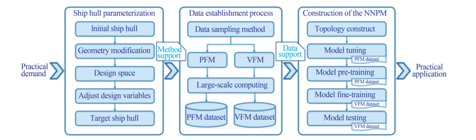Figure  1  The flow chart of the implementation of the NNPM method

Download: Full-Size Img

2   Ship hull parameterization

2.1   The initial hull model

The ship hull parameterizations method adopted in this paper is the semi-parametric method which takes a benchmark hull as the initial hull and parametric its deformed hull based on a set of geometric modification parameters. The initial ship hull adopted in this paper is the Kriso container ship (KCS) hull (Zhang, 2010; Peng et al., 2014). The KCS is a mainstream container ship type developed by the Korean Maritime and Ocean Engineering Research Institute (MOERI, formerly KRISO). The most representative feature of the KCS is its pronounced bulbous bow area which was designed to counteract the resistance-increasing effects of waves. The KCS is also a benchmark hull for method validation due to its open experimental and structural data. To simplify the verification of the adopted CFD method, the KCS model used in this paper is a scale model with a scale ratio of 1∶31.6. The principal parameters of scaled KCS hull geometry are shown in Table 2.

2.2   Hull geometry modification method

The geometry modification method adopted in this paper is the radial basis function (RBF) interpolation technique. Based on the RBF interpolation technique (Buhmann, 2000; Forti and Rozza, 2014), we can achieve a high degree of free deformation of the hull geometry based on control points. The control points in RBF interpolation can be placed anywhere, which gives us the feasibility to deform the target local area finely by performing localized control points refinement. The relationship between the control points with the target points is shown in Eq. (1).

where p(x) is low-degree polynomial term, $\mathcal{N}_c$ is total number of control points, $\gamma_i$ is the weight corresponding to the ith control point, $\varphi\left(\left\|\boldsymbol{x}-\boldsymbol{x}_{c_i}\right\|\right)$ is an RBF whose input is the Euclidean distance between the control point position $\boldsymbol{x}_{c_i}$ and the target point x.

As shown in Eq. (1), based on the coordinates of the control points $\boldsymbol{x}_{c_i}$ before and after deformation, all target points will be deformed after calculating polynomial term p(x), weight $\gamma_i$, and radial basis function φ. The RBF can be selected accordingly based on the actual deformation requirements. Several commonly used RBFs include Gaussian spline, multiquadric biharmonic spline, inverted multiquadric biharmonic spline, and thin plate spline functions. By changing the adopted RBF, we can change the way control points affect object points. Except for the RBF, we can also adjust the weight $\gamma_i$ to change the influence of control points on object points. Due to the highly customizable properties, we adopt the RBF interpolation technique as the geometry modification method for ship hull parameterizations.

2.3   KCS hull discrete method

Before the geometry modification process to the bulbous nose, we need to discrete the hull surface into target points to be deformed. In this work, according to the different calculation methods, the methods of discretization of the hull surface into target points are also different. For the PFM, to control the number of calculation meshes and improve the calculation speed, we directly discrete the KCS hull as a set of discrete points located on the hull surface and set the discrete points as target points. The discrete points need to be arranged with appropriate density depending on the hull area. The representation of hull areas such as bow or stern needs a denser discrete point. By adopting discrete points, we save the workload of the meshing process during the PFM-based calculation. The target points of the KCS hull after the discrete process based on the PFM are shown in Figure 2.

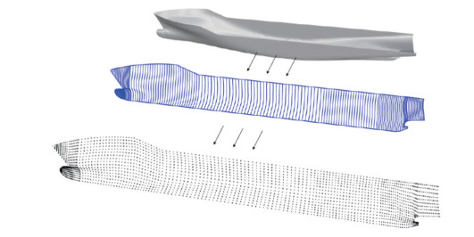Figure  2  The discrete process of the KCS hull of the PFM

Download: Full-Size Img

For the VFM, to achieve a precise representation of the KCS hull, we set the NURBS surface control points as the target points to be deformed. NURBS (Piegl and Tiller, 1996) is a mathematical representation technique that can accurately describe any shape of 3D geometry. Meanwhile, NURBS surface is the primary expression method of the ship hull. NURBS enable us to express the hull surface with arbitrary precision based on a finite number of parameters. Due to the fact that the KCS is an open-source ship form, the NURBS-based KCS model can be obtained easily. The initial NURBS-based KCS surface consists of 110 individual NURBS surfaces. In order to ensure the continuity of the deformation, we merge the NURBS surfaces appropriately. Although the merging process will increase the number of control points, the deformation workload will not increase since we adopt the RBF interpolation technique. The target points of the KCS hull after the discrete process based on the VFM are shown in Figure 3. The hull modification in this paper is conducted based on self-developed in-house code within the computer programming environment of Python, where we realized the deformation of control points or discrete points and the geometric reconstruction of the hull based on control points or discrete points.

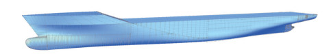Figure  3  The discrete process of the KCS hull of the VFM

Download: Full-Size Img

2.4   Hull geometry modification process and design space

The shape of the bulbous bow area of a ship has a significant impact on the hydrodynamic performance of the ship. In the actual process of optimizing the ship geometry design and optimization, the ship's bulbous bow is also the key target of the optimization and design. In this paper, we focus on the parameterizations of the bulbous bow of the KCS hull, aiming to use appropriate parameters to represent different types and shapes of bulbous noses. The shapes of the initial bulbous bow are shown in Figure 4.

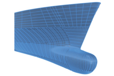Figure  4  The shapes of the initial bulbous bow

Download: Full-Size Img

The geometry modification process can be divided into four stages. Considering that the ship hull is symmetrical, we only describe the location and movement range of control points in the positive direction of the Y-axis. The position and movement of the control points in the negative direction of the y-axis can be obtained by mirroring. The first stage's target is the bulbous bow's cross-section shape. The shape of the cross-section of the bulbous bow can be mainly divided into water drop type, O type, and V type. To enable the cross-section shape of the KCS bulbous bow to deform into these types of cross-sections, as shown in Figure 5, we place two control points that can only move on the Y-axis at the cutting edge of the bulbous bow. In Figure 5, eight fixed control points exist used to define the deformation area. Only the hull part inside the target cuboid formed with eight fixed control points as vertices will be deformed. After several attempts, we set the movement range of control point A as [-0.2, 0.2] and the movement range of control point B as [-0.1, 0.5]. It is well noted that the movement range is an amount normalized based on the target cuboid's length, width, or height. The crosssectional shapes of the bulbous bow in the four extreme cases are shown in Figure 6.

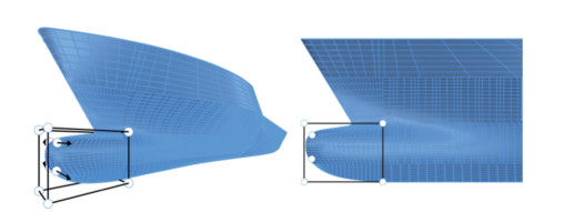Figure  5  Control point arrangement in step 1

Download: Full-Size Img

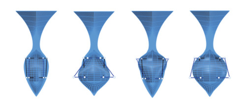Figure  6  The cross-sectional shapes of the bulbous bow in the four extreme cases in step 1

Download: Full-Size Img

The second stage's target is the bulbous bow's middle cross-section shape. The purpose of the second stage is to enable the bulbous bow's middle cross-section shape to deform as water drop type, O type, and V type. As shown in Figure 7, we place two control points that can only move on the Y-axis in the middle of the bulbous nose. To smooth the connection area between the bulbous nose and the after part, we enlarge the length of the target cuboid compared to the first stage. After several attempts, we set the movement range of control point C as [-0.1, 0.1] and the movement range of control point D as [-0.1, 0.1]. The cross-sectional shapes of the bulbous bow in the four extreme cases are shown in Figure 8.

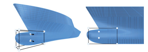Figure  7  Control point arrangement in step 2

Download: Full-Size Img

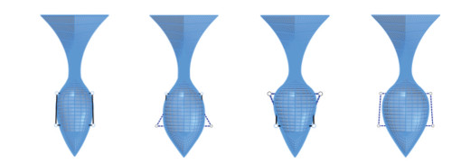Figure  8  The cross-sectional shapes of the bulbous bow in the four extreme cases in step 2

Download: Full-Size Img

The third stage's target is the longitudinal section of the bulbous bow. The third stage's purpose is to enable the bulbous nose's vertex to be moved at the Z-direction. As shown in Figure 9, we place one control point that can only move on the Z-axis in the front end of the bulbous nose. In order to make sure all areas of the bulbous nose are inside the target cuboid, we enlarge the breadth of the target cuboid compared to previous stages. We set the movement range of control point E as [-0.15, 0.1]. The longitudinal section shapes of the bulbous bow in the two extreme cases are shown in Figure 10.

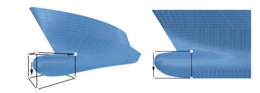Figure  9  Control point arrangement in step 3

Download: Full-Size Img

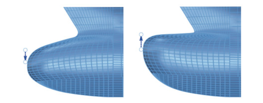Figure  10  The longitudinal section shapes of the bulbous bow in the two extreme cases in step 3

Download: Full-Size Img

The fourth stage's target is the size of the bulbous bow. The fourth stage's purpose is to enable us to change the length of the entire bulbous bow by control points. As shown in Figure 11, we place one control point that can only move on the X-axis in the front end of the bulbous nose. We set the movement range of control point F as [ - 0.1, 0.2]. The longitudinal section shapes of the bulbous bow in the two extreme cases are shown in Figure 12.

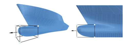Figure  11  Control point arrangement in step 4

Download: Full-Size Img

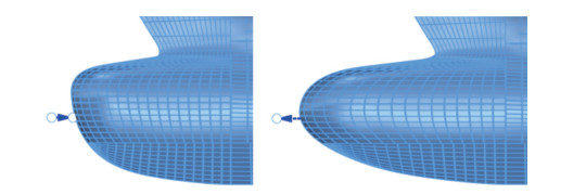Figure  12  Longitudinal section shapes of the bulbous bow in the two extreme cases in step 4

Download: Full-Size Img

The summary of the positions of control points and target cuboid during the four steps of RBF deformation is shown in Table 3. Based on the four steps mentioned above of deformation, we parametric the bulbous nose into six geometric modification parameters, where control points A, B, C, and D are responsible for the representation of cross-section shape, and control points E and F are responsible for the representation of longitudinal section shape. Except for the geometric modification parameters, as shown in Eq. (2), we add a velocity parameter p_v whose range scope is [0.9, 1.1] to change the sailing velocity of the ship, aiming to expand the design space to ships with different sailing velocities. Hence, the final design space is composed of seven different parameters.

where V_d is the sailing velocity of the hull after deformation.

3   Dataset establishment process

The hydrodynamic performance considered in this paper is the total resistance of the ship. For total resistance, we employ PFM and VFM to construct PFM and VFM datasets, respectively. The PFM dataset contains large-scale hull samples used for the tuning and pre-training, and the VFM dataset contains small-scale hull samples used for the fine-training. All the construction processes of the datasets were conducted on a personal laptop computer (Alienware Area-51 m, CPU: Intel Core I9-9900K, 3.60 GHz, RAM: 32.0 GB, and GPU: Nvidia Geforce RTX 2070).

3.1   PFM-based total resistance calculation method

According to the International Towing Tank Conference (ITTC) simplification guideline, the total resistance of a ship in calm water can be divided into wave-making resistance and frictional resistance. This paper adopts Dawson's method (Dawson, 1977; Li et al., 2018) to calculate the wave-making resistance. Dawson's method is one of the most well-known potential flow methods in calculating a ship's wave-making resistance. As shown in Eq. (3), in Dawson's method, the total flow ψ is regarded as the combination of the double-body flow ϕ and wavy flow φ. The double-body flow ϕ satisfies boundary conditions of the hull surface, while the wavy flow φ satisfies both the hull surface and the free surface. Based on the Taylor series, the free surface condition under the sailing velocity of Vcan be written as Eq. (4) after twice expansions.

Since Dawson's method does not consider the fluid viscosity, to calculate the frictional resistance speedy, we employ the classic ITTC friction resistance formula to calculate the ship's frictional resistance. As shown in Eq. (5), the ITTC friction resistance formula adopts the water density ρ, the sailing speed V, the wet surface area S, as well as the friction coefficient C_f calculated based on Reynolds number Re to calculate the friction resistance. The PFM program used in this work is an in-house computer code developed in the authors' laboratory (Li et al., 2018).

3.2   VFM-based total resistance calculation method

In this paper, we employed the commercial tool StarCCM+ (Services, 2021) to apply the Reynolds-averaged Navier-stokes (RANS) approach (Alfonsi, 2009) as the VFM-based total resistance calculation method. We create a virtual towing tank as a computational domain around the target ship. Assuming the length of the water line of the target ship is L, the inlet boundary is set L distance away from the bow, and the outlet boundary is set 2L distance away from the stern. Besides, the side boundary is set 2L distance away from the mid-longitudinal section, the top boundary is set L distance away from the free surface, and the bottom boundary is set 2L distance away from the free surface. We adopt the finite volume method (FVM) as the spatial discretization method to mesh the computational domain.

In order to accurately predict the total resistance of the ship under different complex bulbous bow conditions, we adopted the SST k - ω model, which can simulate the complex flow with strong adverse pressure gradients, as the turbulent model. The free surface method adopted in this paper is the volume of fluid (VOF) method. In order to ensure the accuracy of the ship's resistance under different bulbous bows, the ship's sailing state is not considered in this paper. Considering the purpose of adopting the VFMbased total resistance calculation method is to construct a high-precision dataset, to ensure the accuracy of the VFM dataset, we complete convergence verification of meshing strategy and time step based on KCS hull. All convergence verification cases are conducted under the design velocity of 2.197 m/s for easy validation operation. The benchmark results come from the experimental fluid dynamics, whose total resistance coefficient obtained based on the experiment ranges from 3.56×10^-3 to 3.70×10^-3. Table 4 shows the prediction results for different mesh number cases.

For the mesh number, As shown in Table 4, when we set the mesh number above 460 thousand, the prediction results reach convergence. For the time step, as shown in Table 5, due to the application of the fixed model in the calculation, the time step change has no noticeable effect on the results. Hence, in the following VFM dataset construction, we use the meshing strategy whose mesh number is 540 thousand and set the time step as 0.20 s. As shown in Table 11, under the adopt method setting, we also compare the KCS total resistance result between the PFM, the VFM, and the EFD, where we can find that the VFM shows a higher prediction accuracy than the PFM. The schematic diagram of the domain under the adopted mesh strategy is shown in Figure 13. The wave pattern and the free surface simulated by the VFM calculation are shown in Figure 14.

Figure  13  The schematic diagram of the domain under the adopted mesh strategy

Download: Full-Size Img

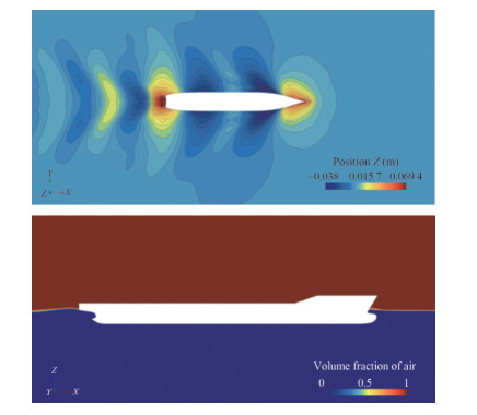Figure  14  The wave pattern and the free surface simulated by the VFM calculation

Download: Full-Size Img

3.3   Hybrid datasets construction

In order to construct an NNPM that can simultaneously achieve high prediction accuracy and a relatively low dataset establishment cost, we need to construct hybrid datasets based on the PFM-based and the VFM-based total resistance calculation methods. Comparing PFM with VFM, it takes about 3 to 5 minutes for a PFM program to complete a case under the computer hardware used by the authors, and due to the low CPU cost, the PFM program can run in parallel on a personal computer. In contrast, the VFM solver takes about 3 to 4 hours to complete a case under the computer hardware used by the authors, and the VFM solver can only run in serial on a personal computer due to the high CPU cost. Hence, inside the hybrid datasets, the PFM dataset will be built for tuning and pre-training, the VFM dataset will be built for fine-training, and the number of hull samples in the PFM dataset will be much larger than that of the VFM dataset.

In this paper, we adopt the grid and the random sampling methods to pick hull samples from the design space to construct the PFM and the VFM datasets. Whether for the PFM or the VFM dataset, the dataset can be further divided into the training, validation, and test datasets. The training dataset helps a neural network model self-update its inner parameters based on a loss function to learn the pattern or mapping relationship that exists in the training dataset. The validation data provides the first test against unseen data, allowing us to evaluate how well models make predictions based on new data. The validation data is the primary evaluation method for the hyperparameters tuning process. The test dataset represents the situation encountered by the model during the actual application process. Based on the test dataset, we can judge the model's generality.

For the PFM training dataset, to ensure that the training samples are evenly distributed in the design space to improve the generality of the NNPM, we adopt the grid sampling method to pick the training samples from the design space. In the process of grid sampling, we interpolate each variable and combine the interpolated points in an enumerated manner to generate hull samples. For the PFM training dataset, the interpolated points of seven variables are shown in Table 7.

Based on the enumeration method, we generated 16 384 hull samples. Based on the PFM, we calculated the total resistance of all 16 384 hull samples to construct the PFM training dataset. Since speed dramatically influences the total resistance, we used continuous uniform distribution to generate 30 000 training samples with random speeds to predict better the relationship between the speed and the total resistance. Considering that the PFM dataset is built for the training and pre-training, we employ the test dataset for both validation and test to save the workload. We used continuous uniform distribution to generate test hull samples to simulate the application situation the NNPM encountered. Finally, we built a PFM training dataset that contains 46 384 hull samples, a PFM validation dataset that contains 5 000 hull samples, and a PFM test dataset that contains 5 000 hull samples.

Same as the PFM training dataset, for the VFM training dataset, we also adopt the grid sampling method to pick the training samples from the design space to ensure that the training samples are evenly distributed in the design space. The grid sampling density of the PFM will be much smaller than that of the VFM. For the PFM training dataset, the interpolated points of seven variables are shown in Table 8.

As shown in Table 8, based on the enumeration method, we generated 192 hull samples. Based on the VFM, we calculated the total resistance of all 192 hull samples to construct the VFM training dataset. Due to the NNPM's topology and hyperparameters already being tuned, during the refining process based on the VFM dataset, the validation dataset is not needed and there only need the test dataset for the final test. Hence, based on the continuous uniform distribution, we built a VFM test dataset containing 40 hull samples.

The schematic diagram of the spatial arrangement of the PFM and VFM data sample is shown in Figure 15. As shown in Figure 15, the blue point represents the PFM data samples, and the cyan-blue represents the VPM data samples. The PFM arrange in the design space with a high density, and the VFM arrange in the design space with a low density. The PFM data sample assists the NNPM in analyzing the mapping relationship in the design space, and the VFM data sample assists in the refinement of the conducted mapping relationship.

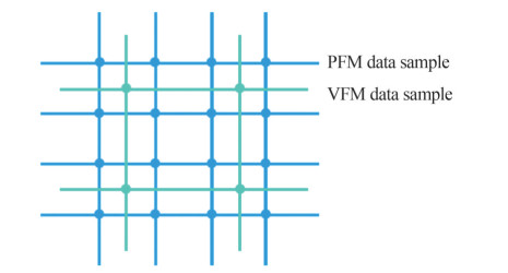Figure  15  The schematic diagram of the spatial arrangement of the PFM and VFM data sample

Download: Full-Size Img

4   Construction of the total resistance NNPM

4.1   Multiple-input neural network

Neural networks (Specht, 1991) are a class of machine learning methods based on artificial intelligence (Dick, 2019). Recently, not limited to its origin field, the neural network technique has outperformed human expert analysis and performance in other fields, including engineering prediction or design. Neural networks have the unique ability to extract patterns or mappings from complex or inaccurate data to find mathematical models that are too complex for the human brain or other computer technologies (Goodfellow et al., 2016). To construct a total resistance NNPM, we need to employ a neural network to extract mapping relationships between the geometric modification and velocity parameters with the corresponding total resistance. After the mapping relationship has been extracted, the NNPM can predict the total resistance automatically and quickly whenever the input changes.

The neural network topology adopted in this paper is the multiple-input neural network (MINN) (Claveria et al., 2015; Huang and Kuo, 2019). The MINN is a deep learningbased parallel computational machine learning method. The main idea of the MINN topology is to construct a neural network that can analyze mixed data, including any combinations of image information, digital information, and category information, in an end-to-end model. An end-to-end topology can keep the continuity of the data flow and further smooth the self-learning algorithm-based tuning and training process. The schematic diagram of the MINN model is shown in Figure 16.

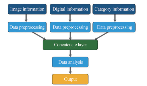Figure  16  The schematic diagram of the MINN model

Download: Full-Size Img

Based on the hull parameterizations process in this paper, the hull with a different bulbous bow under a certain sailing speed has been parametrized as several geometry modification parameters and one velocity parameter. From the perspective of total resistance, the influence of the velocity parameter is much stronger than the geometry modification parameter. In order to deeply uncover the pattern that exists between the geometry modification parameter and the total resistance, we employed additional dense layers to deal with the geometry modification parameter. The schematic diagram of the topology of the NNPM adopted in this paper is shown in Figure 17.

Figure  17  The schematic diagram of the topology of the NNPM adopted in this paper

Download: Full-Size Img

As shown in Figure 17, the NNPM consists of two input layers, two hidden layers, one concatenate layer and one output layer. Expressly, input layer 1 accepts the geometry modification parameters used to describe the shape of the bulbous bow, where each neuron in this layer represents an individual geometry modification parameter from a given sample in the dataset. Input layer 2 accepts the velocity parameter used to describe the hull model's sailing velocity, where only one neuron exists to access the velocity parameter from a given sample in the dataset. Hidden layer 1 was designed for the pre-analyze of the geometry modification parameters. Hidden layer 2 was designed for the analysis of both the geometry modification parameters and the velocity parameter. Two hidden layers are mainly consisting of the dense layer. To construct an end-to-end neural network, we employ the concatenate layer to play a connection function between input layer 2, hidden layer 1, and hidden layer 2. It is well noted that the velocity parameter will be directly imported to the concatenate layer without any processing. Finally, the output layer will export the corresponding total resistance of the current hull model.

4.2   Construction of the MINN model

Except for the topology structure of the neural network, we also need to determine the activation function, loss function, and regularization strategy to build MINN. The activation function can introduce nonlinear properties into neural networks, enabling a neural network to analyze complex problems combining multiple linearity and nonlinearity. We adopted the Parametric ReLU (PReLU) activation and linear activation functions to construct the MINN model to deal with the regression type task. The PReLU activation function (He et al., 2015), whose detail equation is shown in Eq. (6), is a kind of leaky ReLU activation function that can efficiently avoid dying the ReLU problem where all negative values will be ignored. Due to a in Eq. (6) being a trainable parameter, adopting PReLU will increase a neural network's data analysis ability. The linear activation function, whose detail equation is shown in Eq. (7), can accurately output the prediction value of the neural network. The PReLU will be added after every dense layer in the hidden layer, while the linear activation function will be added after the output layer.

The loss function adopted in this paper is the mean absolute error (MAE), whose equation is shown in Eq. (8).

where n is the number of samples in the dataset, y is actual value, $\hat y$ is prediction value.

The regularization strategies adopted in the MINN model include L1, L2 regularization strategies, and the dropout strategy (Srivastava et al., 2014). Considering two kinds of hidden layers exist in the MINN model, we adopt different regularization rates for different parts. The self-learning algorithm adopted in this paper is the Adam learning algorithm (Kingma and Ba, 2014), which can automatically adjust the learning rate during the training process.

4.3   Tuning process of the NNPM

The built MINN can be set as total resistance NNPM. To enable the total resistance prediction ability of the NNPM, we need to complete the tuning and training process of the NNPM. Before the tuning and training process of the NNPM, we normalized the input and output of the dataset separately to make the model easier to converge. As shown in Eq. (9), all input and output variables will be normalized to the range of 0 and 1.

where $v_i^j, \bar{v}_i^j$ are the normalized and raw value variable of the $i$th sample; $v_{\max }^j, v_{\min }^j$ are the ma minimum values of the $j$th variable.

The tuning process of a neural network is one of the most time-consuming processes in constructing a neural network. When tuning the hyperparameters of a neural network, the final prediction performance of the neural network will change as its hyperparameters change. If we regard the final prediction performance of a neural network as output y and regard the hyperparameter combination as input x, a neural network can be regarded as a black box function y = f(x). Each time hyperparameter combination x is input, the prediction performance of the neural network can be obtained after finishing the training process. The tuning process of a neural network can be regarded as finding the hyperparameter combination x corresponding to the neural network with the best prediction performance y in the hyperparameter space.

For the total resistance NNPM, the hyperparameters that need to be tuned include hidden layer structure, regularization rate, and initial learning rate. Due to both hidden layers being constructed by the dense layer, the hidden layer structure can be determined based on the number of dense layers in each hidden layer and the neuron number in each dense layer. The regularization rate includes the L1 regularization rate, L2 regularization rate, and dropout rate. Due to there being two hidden layers, the number of regularization rates that need to be tuned will be doubled. Moreover, considering the number of dense layers might be large, using the grid or random sampling method to search for the best hyperparameter combination will cause a heavy workload.

To reduce the time-consuming tuning process, we use the Bayesian optimizer to assist in the search for the best hyperparameter combination for NNPM. In the Bayesian optimizer algorithm (Snoek et al., 2012), at each iteration, the Gaussian process (GP) (Schulz et al., 2018) will be conducted on the objective function y = f(x) based on historical samples in each iteration. The fitted function y = g(x) obtained by the GP will become the approximated function to assist the optimization process of the objective function y = f(x). With the increase in the iteration number and the number of historical samples, the fitted function y = g(x) will fit closer to the objective function y = f(x), enabling the search for the best hyperparameter combination to be more precise.

We set the dense layer number of hidden layers 1 and 2 from 2 to 10. We set the neuron number in dense layers from 12 to 100 with a gap of 2. For the regularization rate, we set the regularization rate range from 0 to 0.01 with a gap of 5×10^-5. During the tuning process, we set the initial learning rate as 4×10^-5. To ensure every hyperparameter combination is fully tested, we set the maximum training epoch number as 12 000. Meanwhile, we adopt the early stopping strategy (Dodge et al., 2020) to reduce the total tuning workload and set the early stopping patience as 200. For each tuning case, if the validation loss does not decrease after 200 epochs, the training process will be stopped to skip to the following hyperparameter combination. The total tuning trail number is 500. Based on the Bayesian optimizer tuner, we get the optimal hyperparameter combination shown in Table 9. The schematic diagram of the final tuned NNPM is shown in Figure 18.

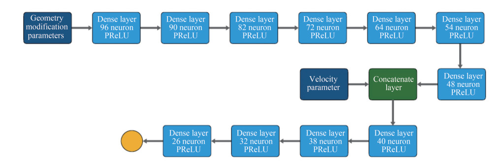Figure  18  The schematic diagram of the final tuned NNPM

Download: Full-Size Img

5   Training and testing of total resistance NNPM

5.1   The pre-training process of NNPM

We can further train the NNPM for better prediction accuracy based on the optimal hyperparameter combination. To accelerate the training process while maintaining precise search, we adopt the stopping and resuming technique to adjust the learning rate during the training process. The pre-training history of the NNPM based on the PFM dataset is shown in Figure 19.

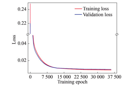Figure  19  The pre-training history of the NNPM based on the PFM dataset

Download: Full-Size Img

As shown in Figure 19, at the beginning of the pre-training process, we set the learning rate as 4×10^-5. The training and the validation loss decreased significantly in the first 7 500 epochs, representing the self-learning algorithm found a specific relationship mapping in the data. We decrease the learning rate to 10^-5 at epoch 12 000. We continue the training process for 12 000 epochs based on the lower learning rate. Finally, we decrease the learning rate to 2×10^-6, where we can find that the training and validation loss keeps decreasing. During the epoch 35 000 to 36 000, we find the validation loss fluctuates between 0.009 71 and 0.009 72 and do not decrease. Hence, we stop the pre-training at epoch 36 000 and store the model in epoch 36 000 as the mathematical model for further refining. In epoch 36 000, the training loss decreased to 8.955×10^-3, and the validation loss decreased to 9.717×10^-3, where we can find that the training loss and validation loss are very close, representing that the pre-trained NNPM does not overfit.

As shown in Table 10, after denormalizing the output, we adopt evaluation metrics, including mean squared error (MSE), root mean squared error (RMSE), mean absolute percentage error (MAPE), symmetric mean absolute percentage error (sMAPE), and the coefficient of determination (R²) (Nagelkerke, 1991), to evaluate the performance of the pre-trained NNPM facing the test dataset. Based on Table 10, we can conclude that the pre-trained NNPM has an outstanding prediction ability. Inside of Table 10, the MAPE value is 0.407%, meaning the average error between the prediction and actual values is 0.407%, showing that the pre-trained NNPM has a very high prediction accuracy from the PFM perspective. The R² value is 0.991, showing the pre-trained NNPM has revealed the mapping relationship between input and output parameters.

5.2   The fine-training process of NNPM

The NNPM obtained based on the PFM dataset can obtain the prediction accuracy of the PFM. The PFM-based NNPM can be used in the assistance of hull design or prediction due to the fast computing power of the NNPM. While the prediction accuracy of the PFM satisfies the accuracy requirements in most cases, we always want NNPM to be as accurate as possible. Once the NNPM can arrive at the accuracy level of the VFM, the AI-based NNPM can be further used in situations where higher precision is required, which further improves the applicability of the NNPM.

In order to better monitor the accuracy changes brought by the fine-training process to the NNPM, we first compare the results of total resistance predicted by different methods to clarify the accuracy gap between different methods. Based on the pre-training NNPM, we predicted every hull sample in the VFM dataset. Meanwhile, we also adopt the PFM to calculate the total resistance of each hull sample in the VFM dataset. Table 11 shows the evaluation metrics between the NNPM predicted values, the PFM predicted values, and the VFM predicted values.

As shown in Table 11, we calculated the evaluation metrics in three different situations: VFM to PFM, PFM to NNPM, and VFM to NNPM. It is well noted that during the calculation of evaluation metrics between A to B, A will be regarded as prediction values, and B will be regarded as actual value. From the situation of VFM to PFM, the MAPE between the PFM and the VFM reaches 5.418%, which shows the differences in forecast accuracy between the two total resistance calculation methods. The R² between the PFM and the VFM reaches 0.843, showing the high fitness between the PFM and the VFM. From the situation of PFM to NNPM, we can conclude that, for the VFM dataset hull samples, the prediction value of the pre-trained NNPM is closer to the prediction value of the PFM, which further proves the pre-trained NNPM has an excellent prediction accuracy from the PFM perspective. From the situation of VFM to NNPM, we can conclude that the prediction values between the NNPM and the VFM also exist the same amount of error with the error between VFM to PFM due to the NNPM being training based on the PFM, which also proves the regression power of the pre-trained NNPM to mapping relationship of the PFM.

To refine the prediction accuracy of the NNPM, we conduct the post-training process on the NNPM based on the VFM dataset and wish to increase the prediction accuracy level of the NNPM to the VFM.

During the fine-training process of the NNPM, we set the VFM training dataset as the training data and the VFM test dataset as the test data. Due to the hyperparameters of the NNPM having been determined based on the PFM dataset, no validation dataset participation is required during the fine-training process, which also saves the dataset establishment workload for us. During the fine-training process of the NNPM, we keep all hidden layers of the NNPM trainable. Although freezing several hidden layers can reduce the number of parameters to be trained in the neural network, freezing parts of hidden layers will break the derived mapping relationship of the NNPM. Since the pre-trained NNPM already reveals the mapping relationship between input and output, we only need to correct the result by post-training to make the result more accurate. Hence, we keep all hidden layers in the NNPM trainable and wish the overall forecast accuracy capability can be improved.

Due to the high computing cost of the VFM, the number of hull samples in the VFM dataset is usually limited. Finetrain the NNPM with a limited number of samples requires appropriate adjustments to the training process. For the NNPM, considering the total trainable parameter number reaches 39 995, we fine-train the NNPM with a low training rate to avoid overfitting. Meanwhile, during the fine-training process of the NNPM, we evaluate the test loss in each iteration and stop the fine-training process when the model is about to overfit. The fine-training history of the NNPM is shown in Figure 20.

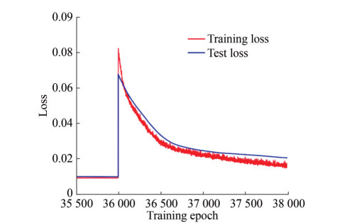Figure  20  The fine-training history of the NNPM based on the VFM dataset

Download: Full-Size Img

As shown in Figure 20, we continue the fine-training process based on the pre-training process. In epoch 36 001, we replace the PFM dataset with the VFM dataset, where we can notice a rapid surge in training and testing loss, representing the different prediction accuracy between the PFM and the VFM. Although the training and testing loss significantly increased, the loss values still keep less than 0.12, representing the regression power of the pre-trained NNPM to mapping relationship in the PFM dataset. Based on the VFM training dataset, we fine-train the NNPM to improve the prediction accuracy of the total resistance NNPM. From epoch 36 001 to epoch 36 500, the training and testing loss decreased significantly. After epoch 36 500, the rate of decline of the loss function value starts to decrease. After epoch 37 500, although the training and testing loss keeps decreasing, the gap between the training and testing loss begins increasing, representing the occurrence of overfitting. We stop the fine-training process at epoch 38 000 to avoid the exacerbation of overfitting. Although we can continue with the fine-training process to reduce the test loss value, we stop the fine-training when the overfitting just appeared to avoid the destruction of the mapping relationship in the NNPM by small dataset overtraining. Finally, as shown in Table 12, we adopt evaluation metrics to judge the predictive ability of NNPM before and after the fine-training process facing the VFM test dataset. As shown in Table 12, the prediction ability of the NNPM shows a signification refinement after the fine-training process.

Table 13 presents the offsets of control points and the velocity parameter, along with the corresponding actual resistance coefficient y, predicted resistance coefficient $\hat y$, and error e, for a randomly selected subset of cases in the VFM test dataset. These results demonstrate the accuracy of the fine-trained NNPM model achieved VFM-level accuracy. We observed that the errors for the cases shown in Table 13 are relatively small, providing strong evidence of the efficacy of our approach. Overall, throughout the section, we presented an NNPM model that can reach the prediction level of VFM while maintaining a reasonable construction cost.

6   Conclusions

In this work, we have developed a high-precision total resistance NNPM based on hybrid datasets while gaining the dual advantages of the low computing cost of the PFM and the high calculation accuracy of the VFM. To summarize this procedure, we first find the geometric deformation of the bulbous bow's cross-section and longitudinal section shape, representing the bulbous bow located in the design space into a set of geometric modification parameters. Based on the calculation data obtained via the bulbous bow representing method, we construct the PFM dataset and the VFM dataset, respectively. In detail, the PFM dataset contains a large number of hull samples, which provide data for the tuning and pre-training processes of the NNPM, while the VFM dataset contains a small number of hull samples, which provide data for the fine-training process of the NNPM.

We employ the multiple-input neural network as the topology structure of the NNPM. Based on the PFM dataset, we first go through the tuning process that required much data to support. Then, based on the PFM dataset, we complete the pre-training process of the NNPM and enable the pre-trained NNPM to obtain the accuracy level of the PFM. Based on the pre-trained NNPM, we finish the finetraining process based on the VFM dataset. The evaluation metrics show that the fine-trained NNPM improves significantly more accuracy than the pre-trained NNPM when facing the VFM method. Meanwhile, the fine-trained NNPM also obtains the accuracy level of the VFM. By simultaneously adopting the PFM and the VFM to construct hybrid datasets, we gain both the fast computation advantage of the PFM and the high accuracy of the VFM during the construction of the NNPM. Since most of the construction process is based on the PFM dataset, the total workload to construct the NNPM is less than that of NNPM using only the VFM. Since the NNPM is refined via the VFM dataset, the accuracy of the NNPM is higher than that of NNPM using only PFM. By adopting hybrid datasets, the NNPM can achieve properties of high prediction accuracy and low construction workload.

Based on the results obtained in this study, we can conclude that the NNPM can predict the ship's hydrodynamic performances with high precision while maintaining an appropriate construction workload. The high precision NNPM can be further used for the prediction of hydrodynamic load in any ship design stage, significantly simplifying the calculation process. We believe that the feasibility of constructing a low-construction workload and high-fidelity neural network proxy model demonstrated in this work will promote the development of artificial intelligence-aided design (AIAD) of a broader class of offshore and navel architectural structures.