
Theoretical Investigation of Spherical Bubble Dynamics in High Mach Number Regimes
https://doi.org/10.1007/s11804-024-00401-w
-
Abstract
The compressibility of fluids has a profound influence on oscillating bubble dynamics, as characterized by the Mach number. However, current theoretical frameworks for bubbles, whether at the first or second order of the Mach number, are primarily confined to scenarios characterized by weak compressibility. Thus, a critical need to elucidate the precise range of applicability for both first- and second-order bubble theories arises. Herein, we investigate the suitability and constraints of bubble theories with different orders through a comparative analysis involving experimental data and numerical simulations. The focal point of our investigation encompasses theories such as the Rayleigh–Plesset, Keller, Herring, and second-order bubble equations. Furthermore, the impact of parameters inherent in the second-order equations is examined. For spherical oscillating bubble dynamics in a free field, our findings reveal that the first- and second-order bubble theories are applicable when Ma≤0.3 and 0.4, respectively. For a single sonoluminescence bubble, we define an instantaneous Mach number, Mai. The second-order theory shows abnormal sensibility when Mai is high, which is negligible when Mai≤0.4. The results of this study can serve as a valuable reference for studying compressible bubble dynamics.-
Keywords:
- Bubble dynamics ·
- Spherical bubble ·
- Cavitation ·
- Compressibility ·
- Mach number
Article Highlights● The suitability and constraints of bubble theories with different orders is investigated.● The single sonoluminescence bubble dynamics is studied theoretically with the instantaneous Mach number.● The bubble radius, bubble surface velocity and the dynamic pressure of the surrounding flow field is studied numerically and theoretically. -
1 Introduction
Bubbles are widely applied in life and industry. They play a crucial role in diverse fields, including naval warfare (Hyunwoo et al., 2022; Li et al., 2014; Lu and Brown, 2021; Zhang et al., 2012; Zhang et al., 2011), seabed resource exploration using airgun bubbles (De Graaf et al., 2014; Li et al., 2020; Zhang et al., 2018), ultrasonic cleaning with microbubbles (Mason, 2016; Tuziuti, 2016), ice-breaking with oscillating bubbles (Cui et al., 2018), emulsification and food industry with bubbles in binary immiscible fluids (Li et al., 2023), and advanced medical treatments (Akbar et al., 2021; Johnson, 1994; Kunkle and Beckman, 1983; Ohl et al., 2009). Nonetheless, the studies on oscillating bubbles characterized by high Mach numbers remain relatively scarce. Examples of such bubbles include those generated by deep-water explosions, where fluid compressibility becomes a critical factor needing special attention.
In the realm of bubble dynamics, theories with different orders of Mach numbers have been developed, offering convenient analytical tools. Pioneering work in bubble dynamics theory began with the Rayleigh–Plesset (RP) equation (Plesset, 1949; Lord Rayleigh, 1917), which can predict a spherical bubble oscillation based on the assumption of incompressibility. However, being a zeroth-order Mach number model, the RP equation implies undamped bubble oscillations and neglects energy radiation. Based on this, Herring (1941) introduced a bubble motion equation incorporating a first-order correction to account for the compressibility of the surrounding liquid. Keller and Kolodner (1956) proposed a compressible bubble theory by utilizing the wave equation rather than the Laplace equation. Building upon these advancements, Prosperetti and Lezzi (1986) derived a family of equations that described bubble wall motion with a first-order Mach number correction, encompassing both Herring's and Keller's formulations by modifying the parameter λ. Considering the essential effect of buoyancy and other factors (Zhang et al., 2015; Zhang and Ni, 2013), Zhang et al. (2023a; 2023b) proposed the unified bubble theory, considering various factors such as boundaries, viscosity, bubble interaction, compressibility, buoyancy, and so on, thereby contributing to a deeper understanding of bubble dynamics.
Regarding the second-order bubble theory, Tomita and Shima (1977) derived the second-order bubble motion equation by using the Poincaré–Lighthill–Kuo method to predict the spherical bubble dynamics in a viscous compressible fluid. Subsequently, Fujikawa and Akamatsu (1980) proposed a mathematical formulation accounting for the compressibility of the fluid, non-equilibrium condensation of the vapor, and so on. In addition, Lezzi and Prosperetti (1987) proposed a second-order bubble equation family by using the matched asymptotic expansions method.
There exist limitations to the application of the mentioned bubble theories when the Mach number of the oscillating bubble is relatively high. Moreover, the deviation between the bubble theories with different orders of Mach numbers must be studied further. Moreover, the results obtained from theories of the same Mach number order exhibit deviations due to the diverse mathematical formulations of bubble equations.
In this paper, we examine the applicability of bubble theories with different orders of Mach numbers through a comparative analysis involving experimental data and compressible numerical simulations. This paper is organized as follows. In Section 2, we introduce the bubble theories and numerical methods, providing a verification analysis of our numerical simulations. In Section 3, we study the spherical bubble dynamics by using the Keller equation with the form of enthalpy, second-order bubble theory, and numerical method to examine the applicability of bubble theories for different Mach numbers. In Section 4, we study single sonoluminescence bubble dynamics utilizing bubble theories with different orders of Mach numbers. Finally, Section 5 offers a concise summary of our findings.
2 Theory and numerical methods
2.1 Spherical bubble theories
With the assumption of an ideal and incompressible fluid, spherical bubble dynamics is always studied using the RP equation (Rozhdestvensky, 2022; Zhang and Ni, 2013). To study the bubble dynamics in the fluid considering compressibility, surface tension, and viscosity, the extended RP equations are proposed. Some essential assumptions are employed for a simpler deduction as follows: 1) Gravity is neglected. 2) Flow is irrotational. 3) Mass transfer or thermal effects during the bubble oscillation are ignored. 4) Bubble gas pressure is uniform. Then, the liquid is governed by the equations of continuity and momentum as follows:
$$ \frac{\partial \rho}{\partial t}+\nabla \cdot(\rho \boldsymbol{u})=0 $$ (1) $$ \frac{\partial u}{\partial t}+u \frac{\partial u}{\partial r}+\frac{1}{\rho} \frac{\partial p}{\partial r}=0 $$ (2) where u=ur is the velocity field, and ρ and p denote the density and pressure of the liquid, respectively. In an irrotational flow field, ∇φ =u, wherein φ denotes the velocity potential. Then, the equations of continuity and momentum become
$$ \frac{1}{c^2}\left(\frac{\partial h}{\partial t}+\frac{\partial \varphi}{\partial r} \frac{\partial h}{\partial r}\right)+\nabla^2 \varphi=0 $$ (3) $$ \frac{\partial \varphi}{\partial t}+\frac{1}{2}\left(\frac{\partial \varphi}{\partial r}\right)^2+h=0 $$ (4) where the sound velocity c and enthalpy h in the liquid are defined as
$$ c=\sqrt{\frac{\mathrm{d} p}{\mathrm{~d} \rho}} $$ (q5) $$ h=\int_{p_{\infty}}^p \frac{1}{\rho} \mathrm{d} p $$ (6) At the bubble surface, where r=R(t), the kinematic boundary condition is
$$ u(r=R(t), t)=\frac{\mathrm{d} R}{\mathrm{~d} t}=\nabla \varphi $$ (7) The equation of state (EOS) of the Tait form (Cole, 1948) is used to describe the water medium
$$ \left(\frac{\rho_l}{\rho_{\infty}}\right)^n=\frac{p_l+B}{p_{\infty}+B} $$ (8) Based on this, the explicit expressions of c and h become
$$ c^2=\frac{n\left(p_l+B\right)}{\rho_l}=c_{\infty}^2+(n-1) h $$ (9) $$ h=\frac{c^2-c_{\infty}^2}{n-1}=\frac{c_{\infty}^2}{n-1}\left[\left(\frac{p_l+B}{p_{\infty}+B}\right)^{\frac{n-1}{n}}-1\right] $$ (10) where the empirical constants B=3 049 bar and n=7.15 for water. c∞ denotes the speed of sound in the liquid at infinity, which can be obtained by
$$ c_{\infty}^2=\frac{n\left(p_{\infty}+B\right)}{\rho_{\infty}} $$ (11) The equations mentioned above can be closed with
$$ p_b=p_g-\frac{2 \sigma}{R}-\frac{4 \mu \dot{R}}{R} $$ (12) where
$$ p_g=p_0\left(\frac{R_0}{R}\right)^{3 \gamma}+p_v $$ (13) Here, pg refers to the bubble gas pressure, and the vapor pressure pv=2 338 Pa. σ and μ denote the surface tension and viscosity coefficients of the liquid, and the polytropic exponent 𝛾 is set as 1.25. We ignore the saturated vapor pressure, considering the considerably high non-condensable gas pressure. p0 is the initial bubble pressure, and we define ε =p0 ∕ p∞ as the strength parameter. In this paper, the Mach number (Fuster and Popinet, 2018; Li et al., 2021) is defined as
$$ M a=\frac{\sqrt{\frac{p_0-p_{\infty}}{\rho_{\infty}}}}{c_{\infty}} $$ (14) where the numerator $\sqrt{\left(p_0-p_{\infty}\right) / \rho_{\infty}}$ almost represents the average velocity of bubble oscillation. In this paper, we focus on the bubble dynamics at different Mach numbers; thus, the ambient pressure p∞ and the initial bubble gas pressure p0 can be obtained from Eq. (14) with known Ma and ε:
$$ p_{\infty}=\frac{M a^2 n B}{\varepsilon-1-M a^2 n} $$ (15) $$ p_0=\varepsilon p_{\infty}=\frac{\varepsilon M a^2 n B}{\varepsilon-1-M a^2 n} $$ (16) Based on the simplified matched asymptotic expansions method (Lagerstrom and Casten, 1972), Prosperetti and Lezzi (1986) presented a bubble wall motion equation family with the first order of the Mach number:
$$ \begin{array}{l} {\left[1-(\lambda+1) \frac{\dot{R}}{c_{\infty}}\right] R \ddot{R}=\frac{3}{2}\left[1-\frac{1}{3}(3 \lambda+1) \frac{\dot{R}}{c_{\infty}}\right] \dot{R}^2=} \\ \;\;\;{\left[1+(1-\lambda) \frac{\dot{R}}{c_{\infty}}\right]\left(h_b-\frac{p_v}{\rho_{\infty}}\right)+\frac{R}{c_{\infty}} \frac{\mathrm{d}}{\mathrm{d} t}\left(h_b-\frac{p_v}{\rho_{\infty}}\right)} \end{array} $$ (17) where hb denotes the enthalpy at the bubble surface, and pv refers to the vapor pressure. When λ=0 and 1, Eq. (17) reduces to the Keller and Herring equations in the form of enthalpy, respectively. We will compare the equations with different λ values in the later section.
Based on the rigorously matched asymptotic expansions method, the second-order bubble motion equation family (Lezzi and Prosperetti, 1987) can be obtained as follows:
$$ \begin{gathered} {\left[1-(\lambda+1) \frac{\dot{R}}{c_{\infty}}+\left(\frac{14}{5}+2 \lambda+\theta\right) \frac{\dot{R}^2}{c_{\infty}^2}\right] R \ddot{R}+\frac{3}{2}\left[1-\left(\lambda+\frac{1}{3}\right) \frac{\dot{R}}{c_{\infty}}+\left(\frac{16}{15}+\frac{4}{3} \lambda+\theta\right) \frac{\dot{R}^2}{c_{\infty}^2}\right] \dot{R}^2+\frac{R^2 \ddot{R}^2}{c_{\infty}^2}=} \\ {\left[1+(1-\lambda) \frac{\dot{R}}{c_{\infty}}+\theta \frac{\dot{R}^2}{c_{\infty}^2}\right] h_b+\left[1-(1+\lambda) \frac{\dot{R}}{c_{\infty}}\right] \frac{\dot{R}}{c_{\infty}} \dot{h}_b} \end{gathered} $$ (18) where λ and θ are arbitrary parameters. More details about the derivation can be found in the reference (Lezzi and Prosperetti, 1987; Prosperetti and Lezzi, 1986).
Regarding a spherical bubble oscillation, the surrounding flow field is symmetric about the bubble center. The bubble oscillation will disturb the surrounding flow field, and the pressure of the liquid can be obtained from
$$ p_l=\rho\left(\frac{2 R \dot{R}^2+R^2 \ddot{R}}{r}-\frac{1}{2} \frac{R^4 \dot{R}^2}{r^4}\right) $$ (19) where r is the distance between the bubble center and the measurement point.
2.2 Numerical method
We use the multiphase solver compressibleInterFoam implemented in OpenFOAM to predict the bubble dynamics in a compressible free field. The equations are discretized and solved using the finite volume method (FVM). The volume-of-fluid method is used to capture the gas-liquid interface and simulate the bubble oscillation. Notably, the bubble dynamics in a free field can be reduced to an axisymmetric problem to improve the computational efficiency. In this paper, the computational domain is shaped like a wedge, as shown in Figure 1. Regarding the boundary conditions on the right-hand side, top, and bottom of the domain, we employ zeroGradient and pressureInletOutletVelocity for pressure field p and velocity field U, respectively. The front and back planes of the wedge-shaped domain are applied with the wedge boundary condition. The left boundary of the wedge forms the axis. In this paper, the domain boundaries are placed around 200 times the maximum bubble radius away from the bubble center to prevent the influence of the reflected wave.
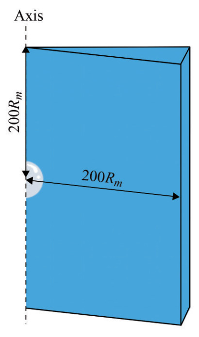 Figure 1 Computational domain for the numerical simulation
The heat and mass transfer, as well as the phase change between the gas and liquid phases, are negligible, then the governing equations become
$$ \frac{\partial \rho}{\partial t}+\nabla \cdot(\rho \boldsymbol{u})=0 $$ (20) $$ \frac{\partial \rho \boldsymbol{u}}{\partial t}+\nabla \cdot(\rho \boldsymbol{u} \boldsymbol{u})=-\nabla p+\nabla \cdot s+\boldsymbol{f} $$ (21) where u refers to the fluid velocity vector, s and f are the viscous stress tensor and surface tension, respectively.
The surrounding liquid follows the Tait EOS mentioned before, and the bubble content is described by the polytropic EOS as follows:
$$ \frac{p_b}{\rho_g^r}=\frac{p_{\infty}}{\rho_{\infty}^r} $$ (22) where the reference density of the liquid ρ∞ =998 kg/m3, density of the bubble gas ρg=1.29 kg/m3, and specific heat ratio r=1.25. During the calculation, the maximum Courant number is set as 0.1 to maintain stability.
2.3 Verification analysis
Before the series of simulations at different Mach numbers, we verify the numerical results by studying a low Mach number case (Ma=0.03) with both theoretical and numerical methods. When the Mach number is sufficiently low, the compressible bubble theories are reliable. We set λ=1 and θ=0 for the second-order bubble equation, i.e., the Tomita and Fujikawa form (Fujikawa and Akamatsu, 1980; Tomita and Shima, 1977). The comparison of the second-order equations with different λ values will be shown later. The Keller form written in terms of enthalpy has been verified as the most accurate first-order equation, which is studied in the reference (Prosperetti and Lezzi, 1986) in detail. In this case, the initial bubble radius is 3 mm, ambient pressure p∞ is 217 720 Pa, and the strength parameter is set as p0=10p∞.
Figure 2 illustrates the temporal evolution of the bubble radius during the two initial periods of oscillation. LPE denotes the second-order Prosperetti & Lezzi equation. The remarkable agreement between theoretical predictions and numerical simulations proves the precision of the numerical method. The bubble radius reaches 0.008 m in the first oscillation period. Due to energy dissipation, the maximum bubble radius during the second period Rm2 is approximately 4.4% smaller than Rm1. Figure 3 shows the dynamic pressure variation in the flow field at a fixed point r= 0.015 m. The pressure peak is related to the minimum bubble radius, and it falls following the attenuation of the bubble oscillation. In conclusion, when the acoustic influence is relatively weak, our numerical results exhibit an exceptional degree of concurrence with both first- and second-order theoretical predictions for a spherical oscillating bubble. This congruence underscores the reliability and credibility of our numerical model.
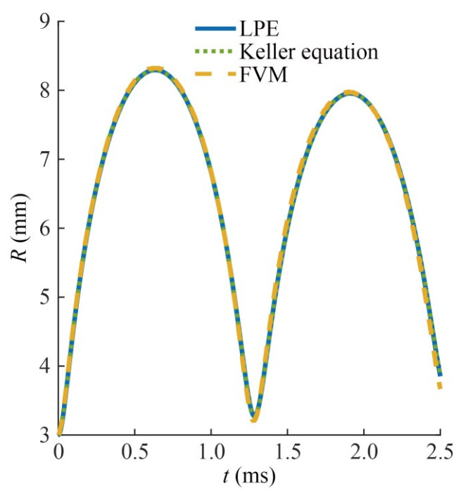 Figure 2 Bubble radius when the Mach number is 0.03
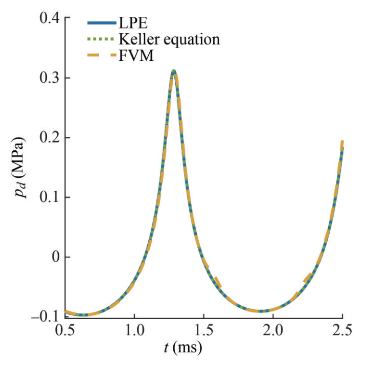 Figure 3 Dynamic pressure of r = 5R0 in the fluid field
3 Spherical bubble dynamics
It is efficient and convenient to study the spherical bubble dynamics using bubble theories. However, as weakly compressible methods, the limitations emerge in their applicability when confronted with relatively high Mach number cases. The objective is to delineate the boundaries of their utility through a rigorous comparison between theoretical predictions and numerical simulations.
The second-order bubble wall equation family (Lezzi and Prosperetti, 1987) encompasses a range of equations distinguished by varying parameters. We conduct a comparative analysis, pitting the outcomes derived from the equations featuring distinct parameter sets (Fujikawa and Akamatsu, 1980; Tomita and Shima, 1977; Wang et al., 2021) against those obtained through numerical methodologies. Specifically, we fix the Mach number at 0.6 for this investigation. As shown in Figure 4, the results reveal a degree of deviation, particularly evident at the maximum bubble radius. Notably, among the considered parameter sets, the theoretical result with λ=1 is the closest to the numerical result (see inset). Thus, we employ the second-order equation with λ=1 (Tomita and Fujikawa form) in this section.
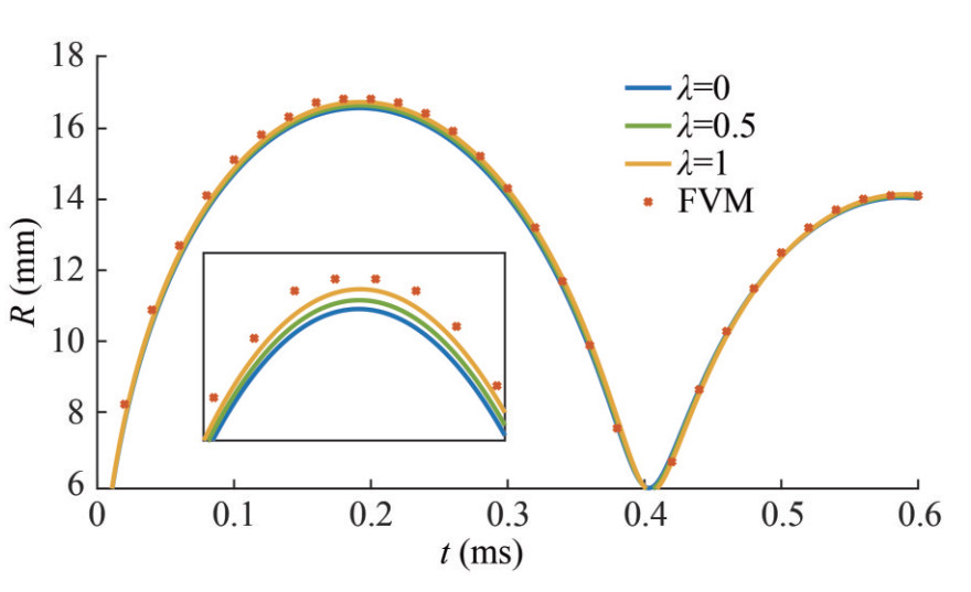 Figure 4 Comparison of bubble radius curves between the numerical simulation and second-order equations with λ =0, 0.5, and 1. The Mach number of this case is set as 0.6
We study the cases with Ma=0.1–0.6 using the first- and second-order theories and the numerical method. The initial bubble radius is set as 3 mm, and p0=100p∞ in all the cases. Figures 5–7 demonstrate the comparison of various bubble dynamics between the numerical and theoretical results. In this section, the Keller equation refers to the equation written in terms of enthalpy. Accordingly, Tables 1–3 present the bubble dynamic behavior at different Mach numbers, demonstrating deviations between the theoretical and numerical results, where ε1 and ε2 denote the deviation between the theoretical result with different orders of Mach numbers and the numerical results. As shown in Figure 5, when Ma≤0.4, the second-order theoretical results closely match the numerical ones, and the deviation is under 0.3%. This suggests that the second-order bubble theory can predict the spherical bubble oscillation precisely when the Mach number is under 0.4. The difference between the second-order theory and numerical results gradually becomes larger when Ma>0.4, reaching about 0.8% and 1% at Ma=0.5 and 0.6, respectively. The first-order theory provides reliable results in a more limited range due to its relatively lower accuracy. The deviation becomes 0.8% when Ma=0.3 and reaches up to 3.2% and 4.3% when Ma=0.5 and 0.6, respectively.
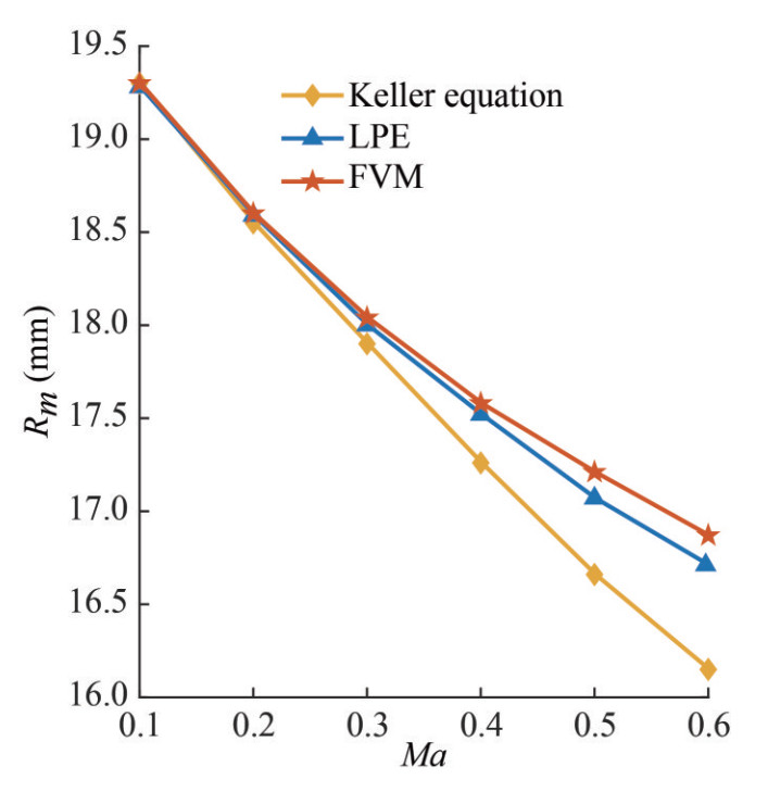 Figure 5 Maximum bubble radius at different Mach numbers
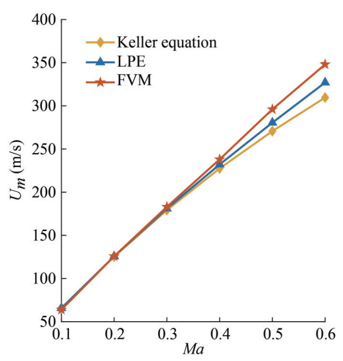 Figure 6 Maximum bubble surface velocity at different Mach numbers
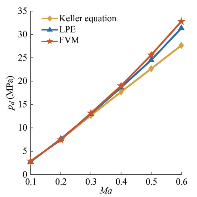 Figure 7 Maximum dynamic pressure in the fluid field at r=5R0 at different Mach numbersTable 1 Maximum bubble radius Rm (mm) at different Ma values
Ma Keller LPE FVM ε1 (%) ε2 (%) 0.1 19.3 19.3 19.3 0 0 0.2 18.55 18.59 18.6 0.3 0.1 0.3 17.9 18 18.04 0.8 0.2 0.4 17.26 17.53 17.58 1.8 0.3 0.5 16.66 17.07 17.21 3.2 0.8 0.6 16.15 16.7 16.87 4.3 1 Table 2 Maximum bubble surface velocity Um (m/s) at different Ma valuesMa Keller LPE FVM ε1 (%) ε2 (%) 0.1 65.73 65.73 65.73 0 0 0.2 125.4 125.7 125.8 0.3 0.1 0.3 179.3 181 183 2 1.1 0.4 227.5 232.1 238 4.4 2.5 0.5 270.7 280.5 296 8.5 5.2 0.6 313.2 327 348 10 6 Table 3 Maximum dynamic pressure pd (MPa) in the fluid field at r=5R0 at different Ma valuesMa Keller LPE FVM ε1 (%) ε2 (%) 0.1 2.74 2.74 2.74 0 0 0.2 7.56 7.52 7.44 1.6 1.1 0.3 12.75 12.98 13.15 3 1.3 0.4 17.7 18.64 19 6.8 1.9 0.5 22.66 24.51 25.59 11.4 4.2 0.6 27.65 31.32 32.77 15.6 4.4 As shown in Figure 6, we can find similar phenomena. For the bubble oscillating velocity, the first- and second-order results gradually deviate from the numerical one as the Mach number increases. The second-order results coincide well with the numerical one when Ma≤0.4, with a deviation under 2.5%. When Ma=0.6, the deviation reaches 6%. For the Keller equation, when Ma≤0.3, the deviation is under 2%, which reaches 4.4% and 10% at Ma=0.4 and 0.6, respectively.
Subsequently, we examine the perturbed flow field surrounding the oscillating bubble. The probe is set at r=5R0 to detect the dynamic pressure, and the initial conditions remain consistent with those previously described. Figure 7 demonstrates the pressure peak in the flow field obtained theoretically and numerically at different Mach numbers. Eq. (19) suggests that the bubble surface velocity plays a vital role in the pressure field, and the bubble oscillating velocity increases dramatically with the Mach number. Thus, the maximum pressure increases with the Mach number due to the higher oscillating velocity despite the smaller bubble volume. When Ma≤0.4, the second-order theory and numerical method yield extremely close results, and the deviation is under 2%. When Ma>0.4, discrepancies become increasingly noticeable, eventually reaching 4.4% at Ma=0.6. For the first-order result, it coincides well with the numerical result when Ma≤0.3, and the deviation is under 2%. At Ma=0.6, the deviation becomes about 16%.
Based on the preceding discussion, we can ascertain the suitability of both first and second-order bubble theories when investigating the dynamics of spherical bubbles within a compressible free flow field. We set 3% as the judgment criterion of the deviation; thus, the first-order theory can simulate the spherical bubble precisely when Ma≤0.3, while the second-order theory is applicable when Ma≤0.4. However, notably, current bubble theories applicable most of the time because high Mach number bubble pulsations are relatively uncommon.
Then, we compare the first- and second-order bubble theories more intuitively. Figures 8 and 9 illustrate the temporal evolution of the oscillating bubble radius calculated by the first- and second-order theories for Ma=0.1 and 0.6. Notably, the pulsation amplitude reduces clearly as the Mach number increases due to higher energy dissipation. In addition, the results of the first- and second-order theories coincide perfectly when Ma=0.1, and the first-order result deviates from the second-order one when Ma=0.6. In an oscillating period, the deviation becomes larger as the bubble expands and becomes smaller when the bubble collapses. Moreover, the deviation generally decreases along the bubble oscillation. The maximum deviations in the first and third periods are 3.6% and 1.6%, respectively; thus, the results coincide better in latter periods than in the first period.
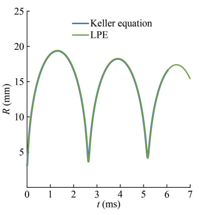 Figure 8 Comparison between first- and second-order bubble radii at Ma = 0.1
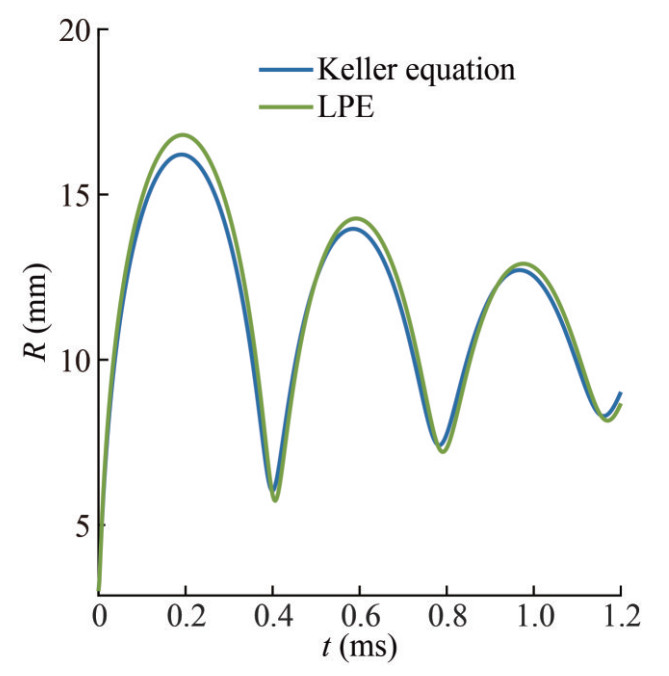 Figure 9 Comparison between first- and second-order bubble radii at Ma = 0.6
4 Sonoluminescence cavitation bubbles
In addition to the bubble oscillating due to considerable pressure difference, another type of cavitation bubble oscillates due to acoustic wave stimulation. Notably, the Mach number reaches exceptionally high levels instantaneously during the rebounding phase of a sonoluminescence bubble. In this section, we study the sonoluminescence cavitation bubbles to compare the capability of different bubble theories of the zeroth-, first- and second-order. In addition, for the second-order bubble theory, different λ values lead to different results; thus, we compare the results of different constant parameter λ values with the experimental data to choose a more reliable form. Moreover, regarding the firstorder theories, discrepancies emerge between the predictions of the Keller and Herring equations, necessitating a comparative evaluation.
We study a single sonoluminescence cavitation bubble using the RP equation, Keller equation, Herring equation, and the second-order bubble theories with λ=1 and 0. The initial bubble radius is set at 4.7 μm, and the initial bubble gas pressure is equal to the pressure at the bubble surface, as shown below:
$$ p_0=p_{\infty}+\frac{2 \sigma}{R}+\frac{4 \mu \dot{R}}{R} $$ (23) where the surface tension and fluid viscosity are set as σ= 0.075 N/m and 0.001 Pa·s, respectively. The bubble is stimulated by the high-frequency acoustic wave set from t=0:
$$ p_{\text {acoustic }}=-P_a \sin (2 \pi f t) $$ (24) where Pa=136 kPa and f=29 kHz. The bubble gas pressure can be obtained by
$$ p_g=p_0\left(\frac{R_0}{R}\right)^{3 \gamma}+p_v $$ (25) where the polytropic exponent is γ=1.4.
The comparison of the sonoluminescence bubble radii between the experimental data from Matula (1999) and the theoretical results are shown in Figure 10. The bubble radius expands to the maximum value of 40 μm at about t=28 μs and then collapses. We can find that all theoretical results coincide well with the experimental result in the first oscillating period. The maximum bubble radius in the second period Rm2 is about 11 μm, 72% smaller than the first period due to the severe energy dissipation. RP equation does not consider the fluid compressibility; thus, the major part of energy dissipation is ignored, and the result deviates dramatically from the experimental data in the second period. Unexpectedly, the second-order theory shows great sensibility. When λ=1, it overestimates the bubble radius in the second oscillating period, with 71% higher Rm2 compared with the experimental one. However, when λ=0, the second-order result coincides well with the experimental data. The sensibility of the second-order bubble theory will be discussed later. In addition, both the Keller and Herring results show good accuracy.
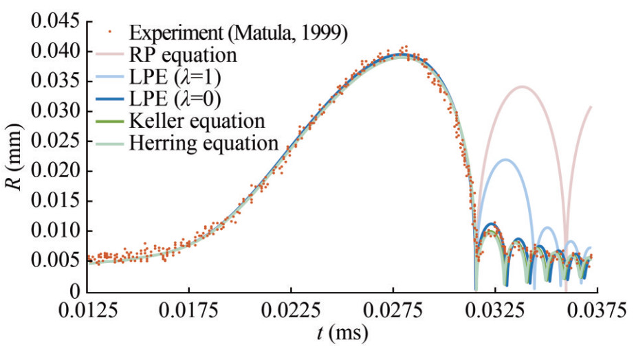 Figure 10 Comparison of the sonoluminescence bubble radii between the experiment and theories with different orders of Mach number
The sonoluminescence bubble is characterized by high oscillating velocity and frequency. Here, we define the instantaneous Mach number Mai=U/c∞ due to the changing ambient pressure; thus, we can focus on the fluid compressibility at every moment. Figure 11 demonstrates the bubble surface velocity obtained from the Keller equation, Herring equation, and second-order theory with different λ values. Evidently, the maximum bubble surface velocity reaches O(103) m/s; thus, the maximum Mai increases dramatically. As discussed before, the second-order equation (λ =0), Keller equation, and Herring equation show good accuracy. However, the second-order equation, which is with a higher order of the Mach number, shows abnormal sensibility. This suggests that the present theoretical frame is not quite suitable in cases with high Mai. In addition, we find some deviations in the bubble velocities between the first and second-order results. The maximum bubble collapsing velocity obtained by the second-order theory is lower than that from the first-order theory, while the maximum rebounding velocity is relatively higher. The second-order bubble rebounds slightly earlier than the first-order one, with a deviation of about 0.09%.
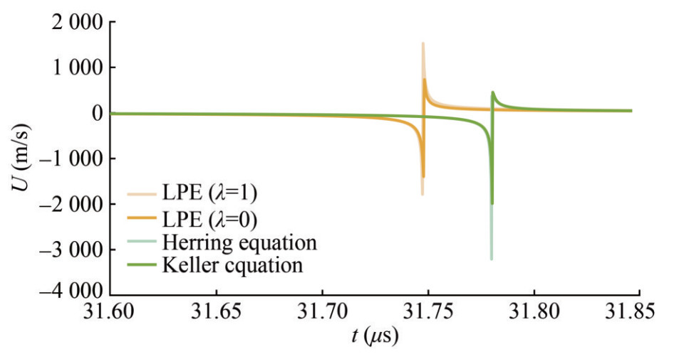 Figure 11 Comparison of the sonoluminescence bubble surface velocity between different bubble theories
To examine the sensibility of the second-order bubble theory, we compare the bubble dynamics between λ =0 and 1. The Mach number is set from 0.01 to 0.7, and other initial conditions remain the same as before. As shown in Figure 12, the relative deviation of the maximum bubble radius of the second period Rm2 increases monotonically with the Mach number, i.e., below 3% when Mai≤0.4. The growth trend gradually becomes stronger when Mai>0.4, and the relative deviation reaches about 22% at Mai=0.7. Accordingly, the bubble radius curves at Ma=0.7 are shown in Figure 13. The results coincide perfectly in the first period, while the deviations about both bubble radius and oscillating frequency emerge from the second period. The bubble oscillation when λ =1 is always stronger than when λ=0, and the same can be found in Figure 10.
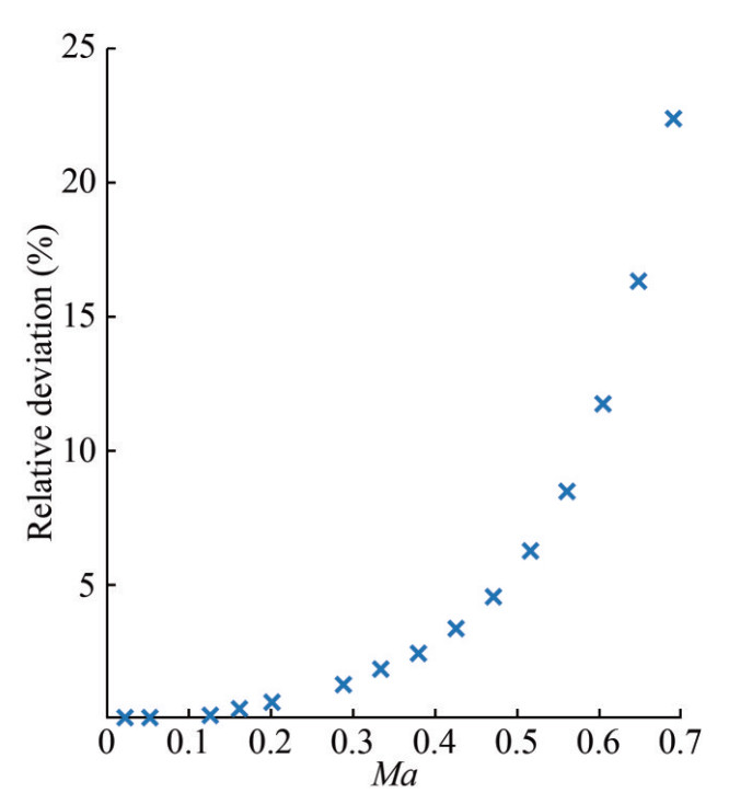 Figure 12 Relative deviation of Rm2 with different Mach numbers
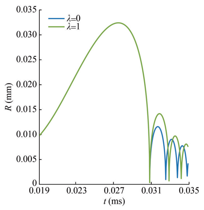 Figure 13 Bubble radius curves when λ=0 and 1
Notably, although the second-order equation (λ =0), Keller and Herring equations can predict the sonoluminescence bubble oscillation well at a high instantaneous Mach number Mai, the second-order theory shows abnormal sensibility. Evidently, this type of sensibility is weak when Mai≤0.4. Overall, the sonoluminescence bubble dynamics must be studied theoretically when the maximum Mai is under 0.4, or the accuracy of the theory must be tested before studying a case at a high instantaneous Mach number.
5 Conclusions
In this study, we have examined the dynamics of spherical bubbles and a single sonoluminescence bubble by employing various bubble theories and numerical simulations. Our investigation has revolved around assessing the applicability and constraints of the first- and second-order bubble theories through comparisons with the FVM simulations and experimental data. The principal outcomes of our research are summarized as follows:
1) The numerical method is validated at a low Mach number. For a spherical bubble oscillating in a free field, the first-order bubble theory is applicable when Ma≤0.3, with the relative deviation from the numerical result under 3%. Beyond the threshold, the deviation increases monotonically with the Mach number. At Ma=0.6, the deviation in the maximum bubble radius and velocity and the dynamic pressure peak reaches 4.3%, 10%, and 16%, respectively.
2) For a spherical bubble oscillating in a free field, the second-order bubble theory is applicable when Ma≤0.4, with a relative deviation under 3%. At Ma=0.6, the deviation in the maximum bubble radius and velocity and the dynamic pressure peak reaches 1%, 6%, and 4.4%, respectively.
3) For a single sonoluminescence bubble, the first-order theoretical result coincides well with the experimental data when the instantaneous Mach number Mai is substantially high, while the second-order theory shows abnormal sensibility. It suggests that the present theoretical frame is not as suitable for high instantaneous Mach number cases. The sensibility of the second-order bubble theory is negligible when Mai≤0.4; thus, the theoretical study is reliable when Mai≤0.4.
In practice, high Mach number (Ma>0.3) bubble pulsations are relatively rare, manifesting primarily in extreme scenarios such as deep-sea detonations and phenomena such as sonoluminescence. Hence, contemporary first- and second-order bubble theories remain applicable in the majority of the cases.
Competing interest The authors have no competing interests to declare that are relevant to the content of this article.Open Access This article is licensed under a Creative Commons Attribution 4.0 International License, which permits use, sharing, adaptation, distribution and reproduction in any medium or format, as long as you give appropriate credit to the original author(s) and thesource, provide a link to the Creative Commons licence, and indicateif changes were made. The images or other third party material in thisarticle are included in the article's Creative Commons licence, unlessindicated otherwise in a credit line to the material. If material is notincluded in the article's Creative Commons licence and your intendeduse is not permitted by statutory regulation or exceeds the permitteduse, you will need to obtain permission directly from the copyrightholder. To view a copy of this licence, visit http://creativecommons.org/licenses/by/4.0/. -
Figure 1 Computational domain for the numerical simulation
Figure 2 Bubble radius when the Mach number is 0.03
Figure 3 Dynamic pressure of r = 5R0 in the fluid field
Figure 4 Comparison of bubble radius curves between the numerical simulation and second-order equations with λ =0, 0.5, and 1. The Mach number of this case is set as 0.6
Figure 5 Maximum bubble radius at different Mach numbers
Figure 6 Maximum bubble surface velocity at different Mach numbers
Figure 7 Maximum dynamic pressure in the fluid field at r=5R0 at different Mach numbers
Figure 8 Comparison between first- and second-order bubble radii at Ma = 0.1
Figure 9 Comparison between first- and second-order bubble radii at Ma = 0.6
Figure 10 Comparison of the sonoluminescence bubble radii between the experiment and theories with different orders of Mach number
Figure 11 Comparison of the sonoluminescence bubble surface velocity between different bubble theories
Figure 12 Relative deviation of Rm2 with different Mach numbers
Figure 13 Bubble radius curves when λ=0 and 1
Table 1 Maximum bubble radius Rm (mm) at different Ma values
Ma Keller LPE FVM ε1 (%) ε2 (%) 0.1 19.3 19.3 19.3 0 0 0.2 18.55 18.59 18.6 0.3 0.1 0.3 17.9 18 18.04 0.8 0.2 0.4 17.26 17.53 17.58 1.8 0.3 0.5 16.66 17.07 17.21 3.2 0.8 0.6 16.15 16.7 16.87 4.3 1 Table 2 Maximum bubble surface velocity Um (m/s) at different Ma values
Ma Keller LPE FVM ε1 (%) ε2 (%) 0.1 65.73 65.73 65.73 0 0 0.2 125.4 125.7 125.8 0.3 0.1 0.3 179.3 181 183 2 1.1 0.4 227.5 232.1 238 4.4 2.5 0.5 270.7 280.5 296 8.5 5.2 0.6 313.2 327 348 10 6 Table 3 Maximum dynamic pressure pd (MPa) in the fluid field at r=5R0 at different Ma values
Ma Keller LPE FVM ε1 (%) ε2 (%) 0.1 2.74 2.74 2.74 0 0 0.2 7.56 7.52 7.44 1.6 1.1 0.3 12.75 12.98 13.15 3 1.3 0.4 17.7 18.64 19 6.8 1.9 0.5 22.66 24.51 25.59 11.4 4.2 0.6 27.65 31.32 32.77 15.6 4.4 -
Akbar A, Pillalamarri N, Jonnakuti S, Ullah M (2021) Artificial intelligence and guidance of medicine in the bubble. Cell & Bioscience 11(1): 1–7. https://doi.org/10.1186/s13578-021-00623-3 Cole RH (1948) Underwater explosions. Princeton University Press. https://doi.org/10.5962/bhl.title.48411 Cui P, Zhang A, Wang S, Khoo BC (2018) Ice breaking by a collapsing bubble. Journal of Fluid Mechanics 841: 287–309. https://doi.org/10.1017/jfm.2018.63 De Graaf K, Penesis I, Brandner P (2014) Modelling of seismic airgun bubble dynamics and pressure field using the Gilmore equation with additional damping factors. Ocean Engineering 76: 32–39. DOI: 10.1016/j.oceaneng.2013.12.001 Fujikawa S, Akamatsu T (1980) Effects of the non-equilibrium condensation of vapour on the pressure wave produced by the collapse of a bubble in a liquid. Journal of Fluid Mechanics 97(3): 481–512. https://doi.org/10.1017/S0022112080002662 Fuster D, Popinet S (2018) An all-Mach method for the simulation of bubble dynamics problems in the presence of surface tension. Journal of Computational Physics 374: 752–768. DOI: 10.1016/j.jcp.2018.07.055 Herring C (1941) Theory of the pulsations of the gas bubble produced by an underwater explosion. Columbia University, New York City Hyunwoo K, Can CB, Joonmo C (2022) Effects of fracture models on structural damage and acceleration in naval ships due to underwater explosions. Ocean Engineering 266(P3): 112930. https://doi.org/10.1016/j.oceaneng.2022.112930 Johnson DT (1994) Understanding air-gun bubble behavior. Geophysics 59(11): 1729–1734. https://doi.org/10.1190/1.1443559 Keller JB, Kolodner Ⅱ (1956) Damping of underwater explosion bubble oscillations. Journal of Applied Physics 27(10): 1152–1161. DOI: 10.1063/1.1722221 Kunkle TD, Beckman EL (1983) Bubble dissolution physics and the treatment of decompression sickness. Medical Physics 10(2): 184–190. DOI: 10.1118/1.595291 Lagerstrom PA, Casten R (1972) Basic concepts underlying singular perturbation techniques. SIAM Review 14(1): 63–120. https://doi.org/10.1137/1014002 Lezzi A, Prosperetti A (1987) Bubble dynamics in a compressible liquid. Part 2. Second-order theory. Journal of Fluid Mechanics 185: 289–321. https://doi.org/10.1017/S0022112087003185 Li S, Saade Y, van der Meer D, Lohse D (2021) Comparison of boundary integral and volume-of-fluid methods for compressible bubble dynamics. International Journal of Multiphase Flow 145: 103834. DOI: 10.1016/j.ijmultiphaseflow.2021.103834 Li S, van der Meer D, Zhang A-M, Prosperetti A, Lohse D (2020) Modelling large scale airgun-bubble dynamics with highly non-spherical features. International Journal of Multiphase Flow 122: 103143. https://doi.org/10.1016/j.ijmultiphaseflow.2019.103143 Li S, Zhang A, Han R (2014) Numerical analysis on the velocity and pressure fields induced bymulti-oscillations of an underwater explosion bubble. Chinese Journal of Theoretical and Applied Mechanics 46(4): 533–543. DOI: 10.6052/0459-1879-13-321 Li S, Zhang A, Han R (2023) 3D model for inertial cavitation bubble dynamics in binary immiscible fluids. Journal of Computational Physics 494: 112508. https://doi.org/10.1016/j.jcp.2023.112508 Lord Rayleigh (1917) On the pressure developed in a liquid during the collapse of a spherical cavity. The London, Edinburgh, and Dublin Philosophical Magazine and Journal of Science 34(200): 94–98. https://doi.org/10.1080/14786440808635681 Lu Z, Brown A (2021) Surrogate approaches to predict surface ship response to far-field underwater explosion in early-stage ship design. Ocean Engineering 225: 108773. https://doi.org/10.1016/j.oceaneng.2021.108773 Mason TJ (2016) Ultrasonic cleaning: An historical perspective. Ultrasonics Sonochemistry 29: 519–523. DOI: 10.1016/j.ultsonch.2015.05.004 Matula TJ (1999) Inertial cavitation and single-bubble sonoluminescence. Philosophical Transactions of the Royal Society of London. Series A: Mathematical, Physical and Engineering Sciences 357: 225–249. https://doi.org/10.1098/rsta.1999.0325 Ohl S, Klaseboer E, Khoo B (2009) The dynamics of a non-equilibrium bubble near bio-materials. Physics in Medicine & Biology 54(20): 6313. DOI: 10.1088/0031-9155/54/20/019 Plesset MS (1949) The dynamics of cavitation bubbles. Journal of Applied Mechanics 16: 277–282. https://doi.org/10.1115/1.4009975 Prosperetti A, Lezzi A (1986) Bubble dynamics in a compressible liquid. Part 1. First-order theory. Journal of Fluid Mechanics 168: 457–478. DOI: 10.1017/s0022112086000460 Rozhdestvensky KV (2022) Dynamics of vapor bubble in a variable pressure field. Journal of Marine Science and Application 21(3): 83–98. DOI: 10.1007/s11804-022-00289-4 Tomita Y, Shima A (1977) On the behavior of a spherical bubble and the impulse pressure in a viscous compressible liquid. Bulletin of JSME 20(149): 1453–1460. DOI: 10.1299/JSME1958.20.1453 Tuziuti T (2016) Influence of sonication conditions on the efficiency of ultrasonic cleaning with flowing micrometer-sized air bubbles. Ultrasonics Sonochemistry 29: 604–611. https://doi.org/10.1016/j.ultsonch.2015.09.011 Wang S, Gui Q, Zhang J, Gao Y, Xu J, Jia X (2021) Theoretical and experimental study of bubble dynamics in underwater explosions. Physics of Fluids 33(12): 126113. DOI: 10.1063/5.0072277 Zhang A, Cui P, Cui J, Wang Q (2015) Experimental study on bubble dynamics subject to buoyancy. Journal of Fluid Mechanics 776: 137–160. https://doi.org/10.1017/jfm.2015.323 Zhang A, Li S, Cui P, Li S, Liu Y (2023a) A unified theory for bubble dynamics. Physics of Fluids 35: 033323. DOI: 10.1063/5.0145415 Zhang A, Ni B (2013) Influences of different forces on the bubble entrainment into a stationary Gaussian vortex. Science China Physics, Mechanics & Astronomy 56: 2162–2169. DOI: 10.1007/s11433-013-5267-2 Zhang A, Shimin L, Cui P, Li S, Liu Y (2023b) Theoretical study on bubble dynamics under hybrid-boundary and multi-bubble conditions using the unified equation. Science China Physics, Mechanics & Astronomy 66(12): 124711. DOI: 10.1007/s11433-023-2204-x Zhang A, Yang W, Yao X (2012) Numerical simulation of underwater contact explosion. Applied Ocean Research 34: 10–20. https://doi.org/10.1016/j.apor.2011.07.009 Zhang A, Zhou W, Wang S, Feng L (2011) Dynamic response of the non-contact underwater explosions on naval equipment. Marine Structures 24(4): 396–411. https://doi.org/10.1016/j.marstruc.2011.05.005 Zhang S, Wang S, Zhang A, Cui P (2018) Numerical study on motion of the air-gun bubble based on boundary integral method. Ocean Engineering 154: 70–80. https://doi.org/10.1016/j.oceaneng.2018.02.008
