1   Introduction

Underwater vehicles such as submarines are important tools for naval requirements, playing a crucial role in offensive operations, targeting military objectives, and conducting reconnaissance because of their notable attributes of high speed, extensive range, and stealth capabilities.

In most previous studies, the DARPA SUBOFF model (Groves et al., 1989) has been widely used as a benchmark model for investigating the flow around an underwater vehicle. A set of experiments (Huang et al., 1992; Jiménez et al., 2010a, b) has been conducted on the DARPA SUBOFF model with or without appendages, and abundant experimental results are offered. Figure 1 shows the fully appended DARPA SUBOFF model, which mainly comprises four parts: the forebody, midbody, stern, and appendages. Underwater vehicles have many typical geometric features. They are usually streamlined, slender, and axisymmetric bodies with changes in curvature in the streamwise and lateral directions. Otherwise, when they navigate, underwater vehicles are usually operated at high Reynolds numbers, Re_L=$\frac{U L}{v}$, based on the hull length L, fluid kinematic viscosity ν, and free-stream velocity U, resulting in a thinner boundary layer relative to the curvature radius. In addition, underwater vehicles are typically equipped with fins, rudders, sails, and other appendages to meet specific operational requirements. The presence of these appendages results in geometric variations on their surfaces.

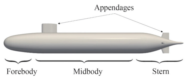Figure  1  Fully appended DARPA SUBOFF model

Download: Full-Size Img

These typical geometric features provide the corresponding flow characteristics for underwater vehicles. The main flow structures at each part are shown in Figure 2.

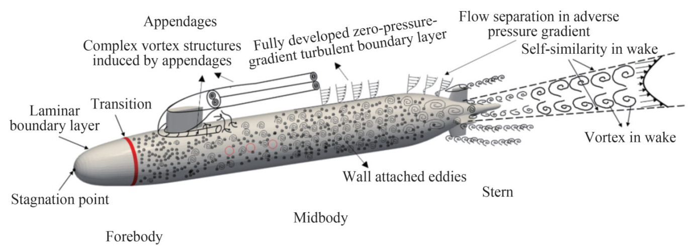Figure  2  Flow structures around an underwater vehicle

Download: Full-Size Img

When an underwater vehicle travels underwater, a stagnation point is generated at the bow head. The flow of the boundary layer over the forebody experiences a laminar stage, a laminar-to-turbulent transition, and finally develops into a turbulent boundary layer (TBL). For the midbody, the wall boundary does not have a streamwise curvature but only a lateral curvature; thus, the streamwise pressure gradient is insignificant. Therefore, the flow is only influenced by the lateral curvature and can be considered a fully developed zero-pressure gradient TBL flow. Wall-attached eddies will also be substantial in this region.

As it develops toward the stern, the flow is influenced by the adverse pressure gradient due to the contraction of the geometric shape. Separation of the boundary layer occurs over the body, resulting in a complex three-dimensional separation flow. Wake will also be generated, leaving behind the stern.

Complex flow structures lead to wall pressure fluctuations and further induce structural vibrations and noise, which have an important effect on the stealth performance of a submarine (Wu et al., 2018; Zhou et al., 2022; Rocca et al., 2022; Balantrapu et al., 2023). Therefore, research on flow structures around underwater vehicles is vital for hydrodynamic performance and the prediction of hydrodynamic noise (Zhao et al., 2022).

This paper aims to provide a review of the latest advances in turbulent flow around underwater vehicles and computational methods for capturing them. Underwater vehicles discussed in this paper are mainly rigid bodies, and the deformation of underwater vehicles is neglected. Research involving the deformation of structures and fluid and structure coupling effects can be found in relevant studies (Merz et al., 2009; Yapar and Basu, 2022). Moreover, underwater vehicles, such as torpedoes, experience cavitation when moving at high speeds, particularly at the edge of the attachment, where vortex cavitation may occur. This occurrence will lead to strong noise and undermine the stealth of the vehicle. However, this paper focused on turbulent flow around underwater vehicles such as submarines, which usually have relatively low speeds and deep navigation positions. Therefore, cavitation flow is usually difficult for submarines to encounter. This field usually involves more complex multiphase flow and bubble dynamics and is not discussed in detail in this paper. More details about this field can be found in relevant studies (Zhang et al., 2017; Gao et al., 2022; Shi et al., 2023; Zhang et al., 2023).

The remainder of this paper is organized as follows. First, flow over the forebody is introduced. The characteristics of the transition and the corresponding computational methods are reviewed. Second, attention is directed toward the flow over the midbody, accompanied by a thorough review of the primary computational methods applied in this context. Third, this paper delves into the intricacies of flow around the stern and wake, presenting relevant research findings and methodologies. Fourth, the flow induced by appendages and the corresponding capturing methods are discussed. Finally, the paper concludes with a summary of the key insights gleaned from the review.

2   Flow over the forebody

For the flow over the forebody, a stagnation point is firstly generated, leading to a peak in pressure at the bow head. The boundary layer over the forebody initiates as laminar and subsequently transitions into a TBL. Notably, most studies in this domain have concentrated on the intricacies of this transition process.

2.1   Boundary layer transition

Boundary layer transition (Figure 3) is a fundamental characteristic of the flow field around the bow of submarine vehicles. This attribute signifies the transformation of the boundary layer flow field from a laminar to a turbulent state. As the flow progresses around the forebody, the Reynolds number of the boundary layer flow gradually increases. Eventually, it reaches a critical value, leading to a transition in the flow field, which ultimately shifts from a laminar state to a turbulent one.

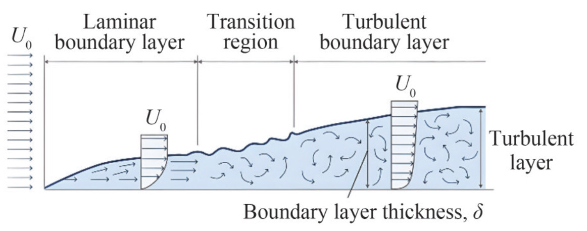Figure  3  Boundary layer transition

Download: Full-Size Img

Boundary layer transition generally comprises three distinct phases: receptivity, linear growth, and nonlinear breakdown leading to turbulence. Receptivity is related to the initiation and excitation of instability waves within the boundary layer. This study addresses the mechanisms by which external disturbances penetrate the boundary layer and emphasizes the reaction of the boundary layer to these external perturbations. The concept of receptivity was initially proposed by Morkovin (1969), and later, Kachanov et al. (1974) explored receptivity by inducing oscillations in the boundary layer through acoustic means. Kachanov (1994) and Borodulin et al. (2002) investigated the receptivity of the boundary layer to three-dimensional disturbances. Perturbation waves, initially motivated by small amplitude external disturbances, undergo a phase of linear growth. This continuous amplification of small amplitude perturbation waves constitutes an inherent mechanism for the transition of the boundary layer. Once the amplitude of these perturbation waves reaches a certain threshold, their evolution becomes nonlinear, ultimately resulting in the breakdown of the flow and the transition to turbulence. Stuart (1958) was the first to investigate nonlinear instability, whereas Craik (1971) extended this research by developing the theory of nonlinear subharmonic stability.

Boundary layer transition is a highly complex flow evolution process that is often influenced by various factors, including wall roughness, free-stream turbulence, pressure gradient, three-dimensional flow, wall temperature, and wall curvature. According to the specific influencing factors, boundary layer transition can be categorized into several main types, including natural transition, bypass transition, separation-induced transition, and crossflow transition.

Natural transition typically occurs in laminar boundary layer flow with a relatively low free-stream turbulence intensity (<1%). As the laminar boundary layer forms at the leading edge of the flat plate and progresses downstream, it is influenced by external disturbances that result in the development of unstable two-dimensional Tollmien–Schlichting (T – S) waves. When the amplitudes of these T – S waves grow sufficiently, they evolve into three-dimensional waves and form vortices. In localized vortex regions, turbulent bursts occur intermittently, resulting in turbulent spots. As these turbulent spots migrate downstream, they continuously entrain the surrounding laminar fluid, causing turbulent spots to gradually expand. Turbulent spots facilitate the full development of turbulence within the boundary layer, ultimately resulting in the transition of the formerly laminar region to a turbulent state (Tang et al., 2019).

Bypass transition typically occurs in laminar boundary layer flow with relatively high free-stream turbulence intensity or high wall roughness. In contrast to natural transition, the environment for bypass transition is characterized by high disturbance levels. These strong environmental disturbances lead to the skipping of the initial evolution stages and the direct generation of turbulent spots within the flow, resulting in an abrupt transition to turbulence.

Separation-induced transition typically occurs in boundary layer flows in the presence of pressure gradients, as illustrated in Figure 4, such as the flow around an airfoil. Under the influence of a strong adverse pressure gradient, the laminar boundary layer experiences velocity reversal, forming laminar separation bubbles. In this scenario, flow instability rapidly intensifies, leading to the transition. Subsequently, these separation bubbles promptly reattach to the wall, at which point the flow state changes to turbulence.

Figure  4  Separation-induced transition around an airfoil (Smith and Ventikos, 2019)

Download: Full-Size Img

Crossflow transition typically occurs in three-dimensional curved surface boundary layer flows, as illustrated in Figure 5, such as the flow around an ellipsoid. Because of factors such as pressure gradients, the boundary layer develops transverse velocity profiles perpendicular to the streamlines. In cases of high free-stream turbulence intensity, crossflow propagates as traveling waves, whereas under lower free-stream turbulence intensity conditions, crossflow instabilities induced by wall roughness become the primary form of instability. Crossflow instabilities, whether stationary or traveling waves, undergo linear amplification followed by nonlinear saturation. During the lengthy nonlinear saturation process, the perturbation amplitudes change very slowly. Nonlinear effects modify the mean flow, leading to secondary instability, and eventually, the rapid growth of secondary instability waves triggers the transition.

Figure  5  Crossflow transition around an ellipsoid (Israeli Computational Fluid Dynamics Center, 2014)

Download: Full-Size Img

The characteristics of boundary layer transition can generally be divided into two aspects: the development of instability wave systems and the formation and evolution of vortex structures. During this process, physical quantities such as velocity and pressure typically undergo considerable pulsation, and at the transition location, the root mean square of the fluctuating pressure often increases.

The development of instability wave systems refers to the process by which the flow becomes unstable because of external disturbances, leading to the development of disturbance wave systems. Flow stability is disrupted, and the transition occurs. The disturbance wave systems undergo a phase of small-amplitude linear growth before entering a nonlinear development phase.

In the later stages of boundary layer transition, after it enters the nonlinear development phase, the flow becomes more disordered and approaches turbulence. The instability waves in the boundary layer transform into dense vortices, including Λ-vortices, hairpin vortices, streaks, and ring vortices. Among these structures, Λ-vortices are the most typical flow structure. The overall evolution of the vortex structures in the later stages of transition can be summarized as follows. As a transition enters the nonlinear development phase, T–S waves, under the influence of nonlinearity, give rise to primary streaks, which are then stretched to form Λ-vortices. Subsequently, Λ-vortices evolve into three-dimensional hairpin vortices, as shown in Figure 6, which induced secondary streaks. The interaction between the primary and secondary streaks generates ring vortices (Figure 7), which eventually develop into a chain-like structure (Figure 8). Although the initial spatial arrangement of Λ -vortices may vary among types of transitions, the overall evolutionary path remains the same (Chen, 2010).

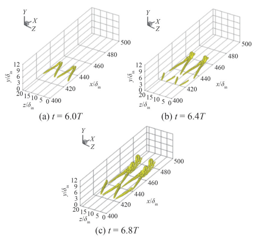Figure  6  Evolution from Λ-vortices to hairpin vortices (Chen, 2010), δ_in is the boundary layer thickness at the inlet

Download: Full-Size Img

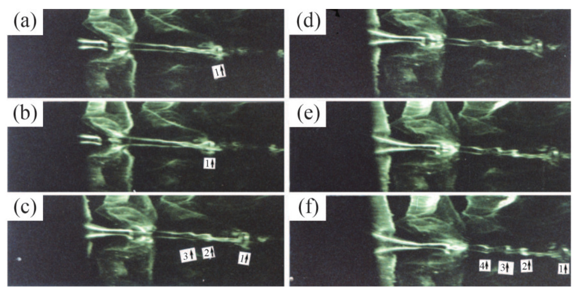Figure  7  Evolution of ring vortices in transition (Lee and Li, 2007)

Download: Full-Size Img

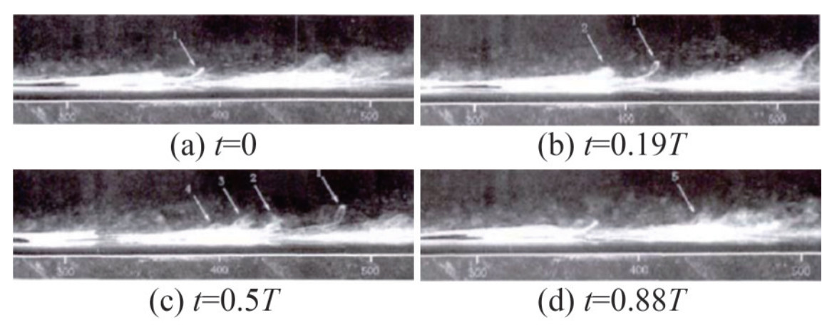Figure  8  Chain-like structure of ring vortices in transition (Guo et al., 2008)

Download: Full-Size Img

2.2   Prediction of boundary layer transition

Three primary methods are used for predicting the boundary layer transition. The first method is the semiempirical method based on linear stability theory (Van Ingen, 1956). The second method is the transition model based on intermittency, which is developed on the basis of the Reynolds-averaged Navier–Stokes model (RANS). The third method involves direct numerical simulation (DNS) and large eddy simulation (LES). It is performed through refined computational fluid dynamics (CFD) to predict the transition.

2.2.1   Semiempirical e^N method

The semiempirical e^N method is a transition prediction method based on linear stability theory (LST). It posits that small disturbances in the boundary layer gradually grow over time or space, with their disturbance amplitude increasing by a factor of e^N. The calculation process can be divided into three main steps:

1) Use LST to express small disturbances in wave form.

2) Solve the eigenvalue problem of the Orr – Sommerfeld equation to obtain the wave number and amplification rate of unstable waves as well as the eigenfunctions.

3) Integrate the amplification rate of unstable waves to obtain the disturbance wave amplitude, represented by the amplification factor N, which is used to predict the transition location.

N in the e^N method is related to the initial disturbance amplitude. However, the physical mechanisms are not entirely clear because the initial disturbance amplitude within the boundary layer is influenced by external disturbance conditions. Therefore, N at the begin of transition is not universal. It needs to be validated through experiments, often falling in the range of 7 to 11.

Recently, many researchers have used the e^N method to predict natural boundary layer transition and analyze transition regions. Mature coupling methods and RANS solvers have been developed for natural transition determination. These methods have been compared and validated with supersonic swept-wing model experiments, demonstrating their applicability in the design of laminar wings for supersonic civil aircraft (Fischer et al., 2021; Nie et al., 2022). Some researchers initially obtained the laminar base flow using a CFD solver, followed by analyzing the stability characteristics of short-nacelle boundary layers under different conditions using LST. Subsequently, they used the e^N method to analyze the transition location and examined the impact of different angles of attack on the boundary layer transition behavior (Niu et al., 2022). Liu et al. (2021) performed flow stability analysis on bow boundary layers over underwater axisymmetric bodies. curved boundary layers. They used the e^N method to predict natural transition locations. The effects of the forebody shapes and the incoming flow velocities on the transition have been investigated.

2.2.2   Transition model based on intermittency

Emmons (1951) proposed that the transition phenomenon is the process of generating spots with turbulent characteristics within the laminar boundary layer. Intermittent behavior was observed across the transitional region as the turbulent spots convected downstream in the boundary layer. These spots formed a rough dynamic sawtooth shape at the interface between the laminar and turbulent flows. The state at each location can be described by the probability of turbulence occurrence. Intermittency γ is defined as the probability that a given point is located inside the turbulent region. Subsequently, many studies have proposed the intermittency model, which can be divided into two methods: algebraic intermittency and transport equations for intermittency. On the basis of the theory of Emmons (1951), Dhawan and Narasimha (1958) used intermittency with an algebraic function to describe the process of transition. Cho and Chung (1992) adopted RANS equations and the k− ε turbulent model and established the k − ε − γ model with the transport equation of γ.

Suzen and Huang (2000, 2001) added the transport equation of γ in the shear stress transport (SST) turbulent model and considered the normal and streamwise directions of γ inside the boundary layer. The model also considered the effect of the pressure gradient, separation, and turbulent intensity of the incoming flow.

Menter et al. (2006) was inspired by the empirical equations of Van Driest and Blumer (1963) and proposed the γ − Re_θ transition model. The γ − Re_θ transition model uses the momentum thickness Reynolds number Re_θ to determine the position of the transition and describes the process of transition with γ. The γ − Re_θ transition model comprises the transport equation for the intermittency and the transport equation for the Reynolds number of momentum thickness. The transport equation for intermittency is expressed as follows:

where U is the fluid velocity, P_γ represents the intermittency generation term, and E_γ represents the intermittency dissipation term. μ_t is the eddy viscosity, and μ is the molecular viscosity. σ_f is the model constant. The expression for the transport equation of $\tilde{R} e_{\theta t}$ is as follows:

where σ_θt is the model constant. By solving the two transport equations of the γ − Re_θ transition model, the distribution of the intermittency can be obtained. It needs to be combined with turbulence models to simulate the transition process. The specific implementation involves using the intermittency factor γ to modify the production, destruction, and blending functions of the SST k − ω turbulence model, as shown in the following equation:

where σ_k is an empirical constant. For the more detailed introduction to the γ − Re_θ transition model, please refer to Menter et al. (2006).

Currently, the transition modified γ − Re_θ transition model is widely used in aerodynamics for transition prediction. It offers high computational efficiency and is applicable to a broad range of transition scenarios. Li (2020) developed a γ − Re_θ transition model within a self-coded CFD program in Fortran. This model was used to numerically simulate various cases, including the flow around multielement airfoils, flow inside turbine cascades, and unsteady flow over wing trailing edges. The results indicated that in the presence of boundary layer transition, the γ − Re_θ model provided more accurate predictions of wall friction coefficients than traditional turbulence models.

Many researchers have also improved the γ − Re_θ transition model based on specific engineering problems. Chen et al. (2017) enhanced the original γ − Re_θ transition model by introducing a modification function in the original correlation function. The new correlation function was implemented in ANSYS-CFX using the CFX expression language. It can accurately predict the transition location of high Reynolds number airfoil boundary layers. Xiang et al. (2021) extended the crossflow mode of the modified γ − Re_θ transition model to create a c − γ − Re_θ transition model suitable for predicting crossflow transitions in high-speed three-dimensional boundary layers. This model was used to predict the crossflow transition on high-speed conical bodies, yielding good agreement with the experimental results. Ye et al. (2023) discovered that under high Reynolds number conditions, the SST γ − Re_θ transition model tended to predict boundary layer transition positions further upstream compared with experimental values. To address this flaw, they used an environmental source term approach to modify the transport equations in the SST γ − Re_θ model. Verification under the condition of high Reynolds number flow over a Donaldson-modified winglet and a NACA 0016 airfoil demonstrated that the modified model improved the accuracy of predicting the boundary layer transition location and other flow field parameters.

2.2.3   Numerical solution method

With the rapid advancement in computer technology, DNS and LES have been applied to boundary layer transition research. DNS directly solves the Navier–Stokes equations and is suitable for investigating the details of various transition phenomena. However, because of the requirement for very fine grids and the current computational capabilities, its application is primarily limited to low Reynolds number flows and relatively simple geometric shapes. LES solves the Navier–Stokes equations on relatively coarse grids and incorporates subgrid-scale (SGS) models to account for unresolved small-scale vortical structures. This is achieved by introducing a SGS viscosity term into the viscous diffusion equations to address the energy dissipation issues of small-scale vortices.

Wang et al. (2016b) provided a detailed description of the physical process from the Λ-vortex to multilevel hairpin vortices. They also proposed that the transition in the flat plate boundary layers is a "vortex construction" process. Zhao et al. (2016) used implicit LES to compute forced transition scenarios. They simulated flow structures using diamond-shaped and ramp-type vortex generators, analyzed the transition process to turbulence in boundary layers, and provided insights into the development of physical quantity fluctuations in the downstream direction. Duan et al. (2014) used DNS to study the transition from laminar-to-turbulent in the subsonic swept-wing boundary layer for a realistic natural-laminar-flow airfoil configuration due to high-frequency secondary instability caused by stationary crossflow vortices. They found good agreement between the predictions from the nonlinear parabolized stability equation and DNS results. Their research also identified rapid increases in the skin friction coefficient and observed a wall shear distribution with a sawtooth pattern during the transition phase. Wang et al. (2018) conducted numerical simulations of boundary layer transition on a flat plate using DNS, investigating boundary layer transition under supersonic inflow conditions and observing the complete evolution of flow transition. Zhou et al. (2019) conducted numerical simulations of spatially developing boundary layers on a flat plate using various SGS models in LES. A comparison was made between different SGS models and DNS predictions of transition position. The results indicate that by observing the distribution of surface friction coefficients along the streamwise direction as a function of the Reynolds number, the transition onset and the point of full turbulence development can be clearly discerned. Furthermore, in the transition region, the velocity profiles exhibited a considerably lower logarithmic layer compared with the profiles in fully developed turbulence, whereas the velocity profiles at the transition peak closely resembled those of fully developed turbulence. Li et al. (2010) conducted DNS of the boundary layer transition on a 5° half-cone-angle blunt cone. The transition location on the cone surface was determined by the rapid increase in the skin friction coefficient. The transition line on the cone surface shows a nonmonotonic curve. The surface friction coefficient contour map provides a clear means of identifying the location of the transition position. Sayadi and Moin (2012) employed six different SGS models with varying grid resolutions to investigate H-type and K-type transitions in zero-pressure gradient boundary layers. They assessed the SGS models' ability to predict transition onset and surface friction throughout the transition process. The results indicated that the SGS models could accurately determine the transition onset location and the laminar and early transitional phases. However, during the later transitional and turbulent phases, the SGS models exhibited less accurate estimations of surface friction because of inadequate shear stress production. Kim et al. (2019) used LES and the parabolized stability equation to simulate the laminar-to-turbulent transition on a flat plate. They validated the accuracy of this coupled method by comparing it with DNS data involving frictional resistance, amplitude growth of instability, and turbulent statistics during the transition process.

Underwater vehicles have more complex geometric shapes, such as axisymmetric bodies, and the boundary layer transition on their surfaces is more complicated than that on flat plates. Consequently, this area has been less researched.

Researchers such as He et al. (2022) employed a stress-blended eddy simulation based on stress to investigate transition phenomena at the bow of a DARPA SUBOFF model at different velocities. They found that during the transition process, pressure fluctuation amplitudes substantially increased before rapidly decaying in the turbulent region and returning to lower levels. Analysis of pressure fluctuation spectra revealed an increase in sound pressure levels within the transition region, with a prominent peak at approximately 100 Hz. Moreover, as the speed increases, the axial pressure fluctuations in the transition region substantially increase, the transition point shifts forward, and the frequency of T-S waves increases.

In numerical studies on the flow of underwater vehicles with a model scale, many scholars (Kumar and Mahesh, 2018a; Morse and Mahesh, 2021; Posa and Balaras, 2016, 2020; Rocca et al., 2022) also employed a numerical disturbance approach at the bow region to artificially induce the transition. The numerical disturbance was usually achieved by adding the steady wall-normal velocity or force source term on the wall boundary on the special position of the forebody. This method will lift the boundary layer and quickly induced the transition of an laminar boundary layer into a turbulent state.

3   Flow over the midbody

Over the midbody of an underwater vehicle, turbulent flow usually reaches full development at high Reynolds numbers, achieving a state of equilibrium in the TBL (Posa and Balaras, 2016). The shape of the midbody can be approximated as a circular cylinder with a constant diameter characterized by lateral curvature and minimal variation in the curvature in the streamwise direction. This attribute results in a flow with almost zero-pressure-gradient effects in the streamwise direction. Therefore, the typical flow characteristic at this location is the fully developed axisymmetric TBL flow in high Reynolds numbers with zero-pressure gradient, as shown in Figure 9.

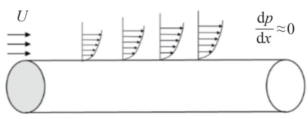Figure  9  Fully developed axisymmetric turbulent boundary layer flow with high Reynolds number and zero-pressure-gradient over the midbody

Download: Full-Size Img

3.1   Zero-pressure gradient turbulent boundary layer

Zero-pressure-gradient turbulent boundary layer (ZPGTBL) flow is one of the most extensively studied fluid phenomena. A recent review by Smits et al. (2011) provided an insightful overview of current findings and future challenges in wall-bounded flows at high Reynolds numbers. This review summarizes the key characteristics of the mean velocity profile and the statistics of turbulent motions. The structure of the TBL is illustrated in Figure 10. Conventionally, the boundary layer comprises an inner region (0<y<0.1δ), where viscosity primarily influences dynamics, and an outer region, where viscosity plays a secondary role in momentum transport processes.

Figure  10  Structure of the turbulent boundary layer (Pope, 2000)

Download: Full-Size Img

For the inner region, the velocity and length scales are based on the wall shear stress τ_w and viscosity ν. The velocity scale is denoted by $u_\tau=\sqrt{\tau_w / \rho}$, representing the friction velocity, and the length scale is characterized by ν/u_τ. The inner region exhibits intense dynamic activity and is divided into three zones: an inner, viscous sublayer (y⁺<5), where turbulence is restrained by the presence of the wall, and the velocity varies as u⁺ =y⁺, where $u^{+}=\frac{u}{u_\tau}$ and $y^{+}=\frac{y u_\tau}{v}$. Then, the buffer layer (5<y⁺<30) is followed and transitions into a logarithmic layer (y⁺>30), where the log law is satisfied:

where κ is Karman's constant and C is a constant, generally approximately 0.39 and 4.9, respectively.

For the outer region, the velocity scale remains u_τ, while the length scale is generally taken as the boundary layer thickness δ. The outer region encompasses the remaining almost 85% of the boundary layer above the log region, which is also known as the wake layer. The velocity profile is described by the defect law

where u_e is the velocity at the edge of the boundary layer. The defect law implies that the momentum deficit, even at a substantial distance from the wall, is sustained by the impact of skin friction. Coles (1956) modeled the outer region as a deviation from the log law and proposed the following law for the wake:

where $W\left(\frac{y}{\delta}\right)$ is the wake function, Π is the wake strength parameter, and κ is the empirical constant.

ZPGTBL involves complex transient and unsteady multiscale motion, nonlinear dynamics, and complex turbulent fluctuations. However, the statistical behaviors of turbulent motions always exhibit a special pattern. All motions are damped right at the surface due to friction and rigidity, and the statistics increase on moving outward, peaking in the inner regions before eventually decaying across the outer region. Otherwise, in the outer regions, the motions are nearly isotropic. The vertical and spanwise normal stresses are approximately equal to the streamwise stresses. For more detailed insights into the statistics of turbulent motions, refer to Smits et al. (2011) and Balantrapu (2020).

Coherent structures play a vital role in the flow characteristics of ZPGTBL. They are integral to statistical properties and substantially contribute to the production, transport, and dissipation of turbulent energy through their formation, interactions, and demise. Coherent structures in ZPGTBL have been extensively investigated in previous studies (Kline et al., 1967; Hutchins and Marusic, 2007; Adrian, 2007; Monty et al., 2007; Wu and Moin, 2009; Wang et al., 2022). Four principal characteristic elements for coherent structures are identified in ZPGTBL as follows:

1) Low-speed near-wall streaks with a typical spanwise spacing of approximately 100ν/u_τ (Kline et al., 1967; Posa and Balaras, 2016; Kumar and Mahesh, 2018a), as shown in Figure 11.

Figure  11  Streaks in near-wall turbulent flow at y⁺=5.6 from the wall (Chernyshenko and Baig, 2005)

Download: Full-Size Img

2) Hairpin or horseshoe vortices of a range of scales starting with a minimum height of 100ν/u_τ (Adrian, 2007), as shown in Figure 12.

Figure  12  Hairpin or horseshoe vortices (Theodorsen, 1952)

Download: Full-Size Img

3) Large-scale motions (LSM) formed by groups of hairpin vortices when multiple hairpin structures travel at the same convective velocity (Adrian, 2007), as shown in Figure 13.

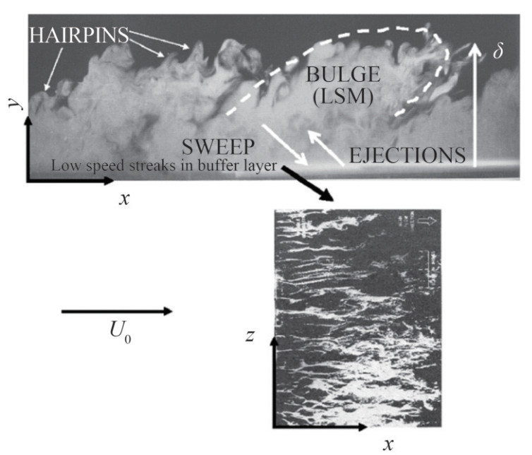Figure  13  Large-scale motions (Adrian, 2007)

Download: Full-Size Img

4) Very large scale motions (VLSM) at high Reynolds number flows, as shown in Figure 14, possibly formed from the streamwise alignment of LSM (Hutchins and Marusic, 2007; Monty et al., 2007).

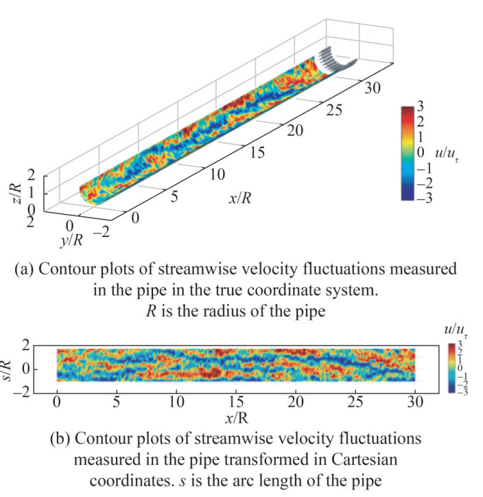Figure  14  Very large scale motions (Monty et al., 2007)

Download: Full-Size Img

3.2   Effects of the lateral curvature

The effects of lateral curvature have been widely investigated by considering axial flow past a constant-radius circular cylinder, excluding any streamwise pressure gradient effects. The common radius-based Reynolds number, Re_a = $\frac{U a}{v}$, where a is the radius of the cylinder, and U is thefreestream velocity, cannot include any effect of the boundary layer or wall shear stress. Therefore, the impact of the lateral curvature is commonly characterized by two popular nondimensional parameters:

1) δ/a, the ratio of boundary layer thickness to the radius of curvature.

2) a⁺ = au_τ /ν, the radius-based Reynolds number in wall units, where u_τ is the skin-friction velocity.

Three flow regimes have been identified on the basis of these parameters (Piquet and Patel, 1999): 1) δ/a and a⁺ are large, 2) large δ/a and small a⁺ and 3) small δ/a and large a⁺. The first flow regime is observed in axial flow over a long thin cylinder at high Reynolds numbers, where the influence of curvature is notable. The second flow regime arises in axial flow over thin cylinders at low Reynolds numbers, where the axisymmetric TBL behaves like an axisymmetric wake, featuring an inner layer characterized by strong curvature and low Reynolds number effects. Most studies in previous literature concentrated on the first two regimes (Piquet and Patel, 1999; Balantrapu et al., 2021). The third flow regime is prevalent in applications where the Reynolds number is high, but the boundary layer is thin compared to the radius of curvature. This flow regime is usually treated as a planar boundary layer because of its similarity to its flat plate counterpart. However, it is essential to recognize that there are considerable fundamental differences between a planar TBL and a thin axisymmetric TBL at high Reynolds numbers. These distinctions include increased skin friction, rapider radial decay in turbulence away from the wall, and fuller velocity profiles due to transverse mixing (Lueptow, 1990; Kumar and Mahesh, 2018b). Kumar and Mahesh (2018b) extended the integral analysis conducted by Wei et al. (2017) to include axisymmetric boundary layers. They derived the mathematical expression for the skin-friction coefficient in axisymmetric boundary layers as Eq. (7) and validated the experimental observation that skin friction increases compared to a flat plate for an axisymmetric boundary layer.

3.3   Numerical simulation methods

3.3.1   RANS method

Because of the cost advantages in computation, the RANS method is widely employed and recommended in the study of time-averaged flow over the midbody. In RANS, the entire range of turbulent flow scales is modeled, and information on velocity and pressure fluctuations is unavailable.

Turbulent models are used to close the solution of the RANS equations. Recently, many famous turbulent models have been proposed and developed. On the basis of the number of equations, turbulent models can be divided into zero-equation models, one-equation models, two-equation models, and seven-equation models. Two-equation turbulent models are widely used in engineering applications, including k − ω model (Saffman and Wilcox, 1974; Robinson and Hassan, 1996), k − ε model (Jones and Launder, 1972; Launder and Spalding, 1974), and SST k − ω model (Menter, 1994), etc. The k − ω model is suitable for low Reynolds numbers and can be directly calculated within the viscous sublayer without the need for a wall function. In contrast, the k − ε model is applicable to high Reynolds numbers but cannot directly solve for the viscous sublayer and transition layer, requiring the use of a semiempirical wall function to describe the transition from the boundary layer to the fully developed turbulent layer outside the boundary layer. The k − ω model accurately predicts flow within the near-wall boundary layer and effectively handles issues such as adverse pressure gradients and flow separation. However, it tends to be overly sensitive to the inlet turbulence parameters in the far-field region. In contrast, the k − ε model performs well in free shear flow problems but exhibits limitations in the presence of large adverse pressure gradients. The SST k − ω model, proposed by Menter in 1974, employs the k − ω model within the boundary layer and a standard k − ε model in the outer region and free flow area. Thisblending is achieved through a mixing function that combines the strengths of both models while mitigating their respective drawbacks.

The RANS method has shown good performance in capturing time-averaged statistical quantities such as the time-averaged pressure coefficient, friction coefficient, and fluid field. Yang and Lohner (2003) used RANS and Baldwin– Lomax turbulence model (Baldwin and Lomax, 1978) to simulate the time-averaged flow around the DARPA SUBOFF with appendages at 0° and nonzero angles of attack. The time-averaged surface pressure, shear vectors, and vorticity contours around the midbody are predicted as shown in Figure 15. The time-averaged pressure and skin-friction coefficients achieved good agreements with the experimental measurements with and without a fairwater at a 0° angle of attack. Boger and Dreyer (2006) used RANS and overset mesh to simulate the flow around the DARPA SUBOFF and ONR Body-1 submarine models. Time-averaged surface pressures and predicted forces and moments around the midbody agreed well with experimental measurements. Toxopeus (2008) conducted RANS to study the bare hull DRAPA SUBOFF sailing straight ahead and in oblique motion. Menter's one-equation turbulence model and two-equation SST k − ω model were used. Good agreements with the experiments were achieved regarding time-averaged pressure and skin-friction coefficients, axial and radial velocities, and Reynolds shear stress. Cao et al. (2016) adopted the k − ω turbulent model to simulate the flow over the bare hull DRAPA SUBOFF model for steady drift tests and rotating arm tests and achieved a good prediction for the time-averaged forces and moments. Similar studies with RANS have been conducted by Gao et al. (2018). However, RANS has difficulty capturing more detailed information about unsteady turbulent flow fluctuations and pressure fluctuations.

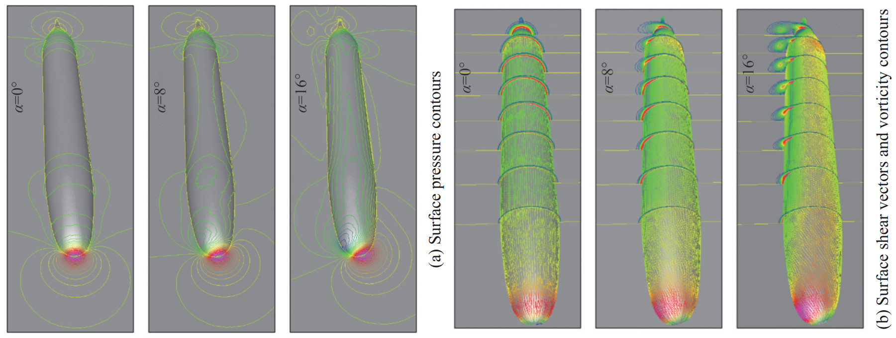Figure  15  Surface pressure contours, shear vectors, and vorticity contours for the DARPA SUBOFF in 8 cut planes at 0°, 8°, and 16° angles of attack (Yang and Lohner, 2003)

Download: Full-Size Img

3.3.2   LES method

In recent decades, LES has evolved into an indispensable engineering tool for predicting and analyzing unsteady, multiscale, and multiphysics turbulent flows. The accuracy of LES approaches primarily stems from the direct resolution, on a computational mesh, of the dynamics of energy-dominant and flow-dependent large eddies, as opposed to relying on modeling.

LES comprises two critical components: the filter and the SGS model. First, a mathematical filtering model is implemented to remove smaller eddies whose scales are beneath the filter function's scale. This process decomposes the instantaneous governing equations into filtered equations, characterizing the behavior of large-scale eddies. Second, the impact of the filtered-out small-scale eddies on the large-scale ones is addressed by introducing an additional stress term, referred to as the SGS stress term, into the governing equations. This mathematical framework is commonly known as the SGS model. The earliest SGS model, proposed by Smagorinsky (1963), is the eddy viscosity model based on isotropic turbulence. It assumes that the SGS viscosity can be expressed as the product of the model coefficient, the relevant length scale, and the relevant velocity scale. The coefficient C_s in this model is a constant value selected empirically. However, because the flow field is dynamically changing and the SGS viscosity v_SGS decreases near the wall, the Smagorinsky SGS model often generates excessive dissipation during computations.

As research has advanced, some scholars have modified the Smagorinsky SGS models by considering flow characteristics near the wall from different perspectives. Notably, Van Driest (1956) introduced the Van Driest damping function to adjust the length scale term of the SGS viscosity near the wall, effectively reducing the SGS viscosity and consequently diminishing dissipation in proximity to the wall. Germano et al. (1991) introduced the dynamic Smagorinsky (DSMAG) model, which was later modified by Lily (1992). The DSMAG model modifies the Smagorinsky model by adjusting the model coefficient. It is based on a specific single-filter model and performs secondary filtering of the flow field. This model adjusts the model coefficient C_s in real-time on the basis of the results of the two filtering operations. This feature allows the coefficient C_s to vary with the changing flow field, demonstrating accurate asymptotic behavior near solid walls and in laminar flows. Nicoud and Ducros (1999) proposed the wall-adapting local eddy viscosity (WALE) model, which is a composite model that considers the effects of turbulence near walls and momentum transfer. The WALE model modifies the strain-rate tensor term in the SGS viscosity, and its primary advantage lies in automatically setting the SGS viscosity to zero in pure shear flow regions, ensuring an accurate simulation of flow fields near the wall.

The previously mentioned SGS models are algebraic eddy viscosity models. Another type of SGS model is known as the one-equation eddy viscosity model. The development of this SGS model is primarily aimed at addressing the limitations of the local balance assumption between energy production and dissipation in algebraic eddy viscosity models, particularly in high Reynolds number flow with insufficient grid resolution. Yoshizawa and Horiuti (1985) first proposed the k-equation SGS (KSGS) model, which considers the transport process of turbulent kinetic energy (TKE) at the subgrid scale. By introducing a transport equation for the SGS kinetic energy, the turbulent motion at the subgrid scale is better represented. The model coefficients C_k and C_ε are constants. In addition, Kim et al. (1997) suggested dynamically adjusting the model coefficients C_k and C_ε based on the flow field and proposed the dynamic k-equation SGS (DKSGS) model. This dynamic adaptationimproves the adaptability and accuracy of the model, allowing it to better accommodate different flow conditions.

In the academic research field, LES has become an indispensable engineering tool for predicting and analyzing unsteady, multiscale, and multiphysics turbulent flows. However, in practical engineering applications, LES is not widely utilized, mainly because of the high computational demands of wall-resolved LES (WRLES) for high Reynolds number flows (Piomelli, 2008). In WRLES, most of the computational grid is dedicated to resolving the inner layer of the boundary layer flow. For the fully developed TBL, the size of the energetic eddies in the inner layer (which occupies approximately 10% to 20% of the boundary layer thickness) is on the order of the viscous length scale δ_ν = ν/u_τ. The outer layer of the boundary layer is characterized by the local boundary layer thickness δ. Their ratio defines the Reynolds number Re_τ = δ/δ_ν based on the friction velocity.

As the Reynolds number increases, the energy-containing scales in the inner layer of the boundary layer decrease. Consequently, to effectively capture the flow dynamics within this inner layer, the grid resolution must match the order of the viscous length scale, leading to computational costs that are frequently impractical. Thus, the fundamental concept behind wall-modeled LES (WMLES) is to directly compute and resolve the flow in the outer layer of the boundary layer, employing modeling approaches for the flow within the inner layer of the boundary layer. Treatments of the flow near the wall for WRLES and WMLES are shown in Figure 16.

Figure  16  Treatments of flow near the wall for WRLES and WMLES (Piomelli, 2008)

Download: Full-Size Img

In terms of computational cost, Chapman (1979) presented a landmark paper that compared and estimated the number of grid nodes N required for DNS and WRLES, emphasizing the importance of wall modeling. Recently, Choi and Moin (2012), building on Chapman's work, reexamined the computational cost issue using more accurate formulas for high Reynolds number boundary layer flows. They specifically focused on comparing the computational costs of WRLES and WMLES. This study showed that the number of grid nodes required for DNS, WRLES, and WMLES is proportional to $N_{\mathrm{DNS}} \sim R e_L^{37 / 14}$, $N_{\text {WRLES }} \sim R e_L^{13 / 7}$, and $N_{\text {WMLES }} \sim R e_L$, where L represents the length of the flat plate. Notably, the computational cost of WMLES exhibits a linear relationship with the Reynolds number, which considerably expands the range of Reynolds numbers that LES can handle.

Posa and Balaras (2016) performed WRLES to simulate the flow around DARPA SUBOFF with appendages at Re_L= 1.2×10⁶. They achieved great agreements with experiments about pressure and skin-friction coefficients and captured instantaneous streamwise velocity fluctuations and near-wall streaks over the midbody, as illustrated in Figure 17. Kumar and Mahesh (2018a) used WRLES to capture the flow around the DARPA SUBOFF without appendages at Re_L=1.1×10⁶. The near-wall flow structures on the hull are visualized using the isocontour of the instantaneous Q-criterion, as shown in Figure 18. They compared the flow over the midbody with the planar TBL and found that the TKE profile of the axisymmetric TBL decays faster than that of the planar TBL. A more rapid decay in fluctuations away from the wall and an increasing skin friction coefficient were also observed compared with planar TBL. Typical near-wall streaks over the midbody were also observed, as shown in Figure 19. The same conclusions were drawn by Morse and Mahesh (2021). They adopted WRLES to simulate the flow over the DARPA SUBOFF model without appendages and provided a new perspective on the analysis of TBL in an orthogonal coordinate system aligned with streamlines, streamline-normal lines, and the plane of symmetry. The wall-attached eddies around the model are shown in Figure 20. ZPGTBL in the midbody was analyzed using an orthogonal coordinate system. They found that the mean advection term was much smaller than that for the laminar profile because of the lack of streamwise pressure gradients over the midbody. The pressure at the wall was equal to the pressure outside the boundary layer because the streamwise-normal pressure gradient balances the streamwise-normal gradient of the streamwise-normal velocity fluctuation term $\bar{u}_n^2$.

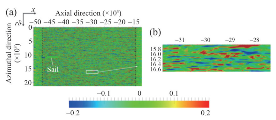Figure  17  Streamwise velocity fluctuations relative to the mean field at 10 wall units from the surface of the midbody (Posa and Balaras, 2016)

Download: Full-Size Img

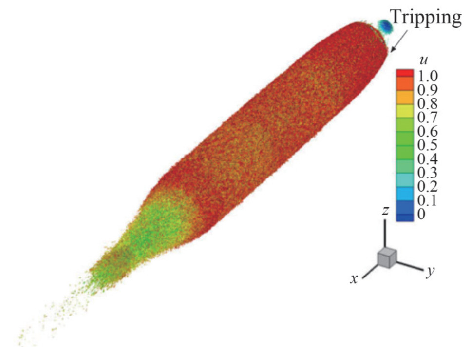Figure  18  Near-wall flow structures on the hull are visualized using the isocontour of the instantaneous Q-criterion (Kumar and Mahesh, 2018a)

Download: Full-Size Img

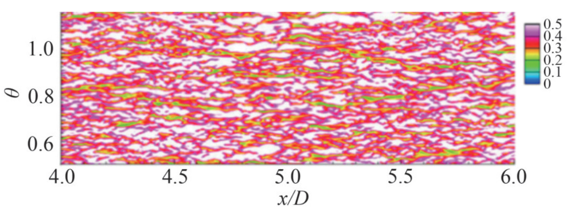Figure  19  Typical near-wall streaks for instantaneous axial velocity distribution over the midbody at approximately y⁺=10 from the hull surface (Kumar and Mahesh, 2018a)

Download: Full-Size Img

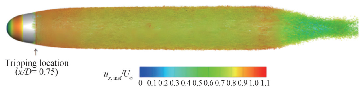Figure  20  Wall-attached eddies with instantaneous isocontour of the Q-criterion (Hunt et al., 1988) colored by instantaneous axial velocity are shown near the hull surface to visualize near-wall structures

Download: Full-Size Img

Otherwise, massively parallel computing is another approach to explore the application of LES in solving the flow in high Reynolds number flows. Recently, Liu et al. (2023) considerably increased the efficiency of massively parallel computing on an unstructured mesh by proposing a geometrical method based on the mesh reordering method using a Hilbert space-filling curve. Their work sets a new record in the Reynolds number (Re_L=1.2×10⁶) and mesh cell number (1.476 billion cells) in WRLES of turbulent flows over SUBOFF on an unstructured mesh, which provided for overcoming the difficulties in LES of high Reynolds number flows without losing the flow details near the wall. Instantaneous flow structures near the wall visualized using the Q-criterion isosurface are shown in Figure 21. Fluctuations in the axial and normal velocities showed satisfactory agreement with previous WRLES work (Kumar and Mahesh, 2018a) and experiments (Huang et al., 1992).

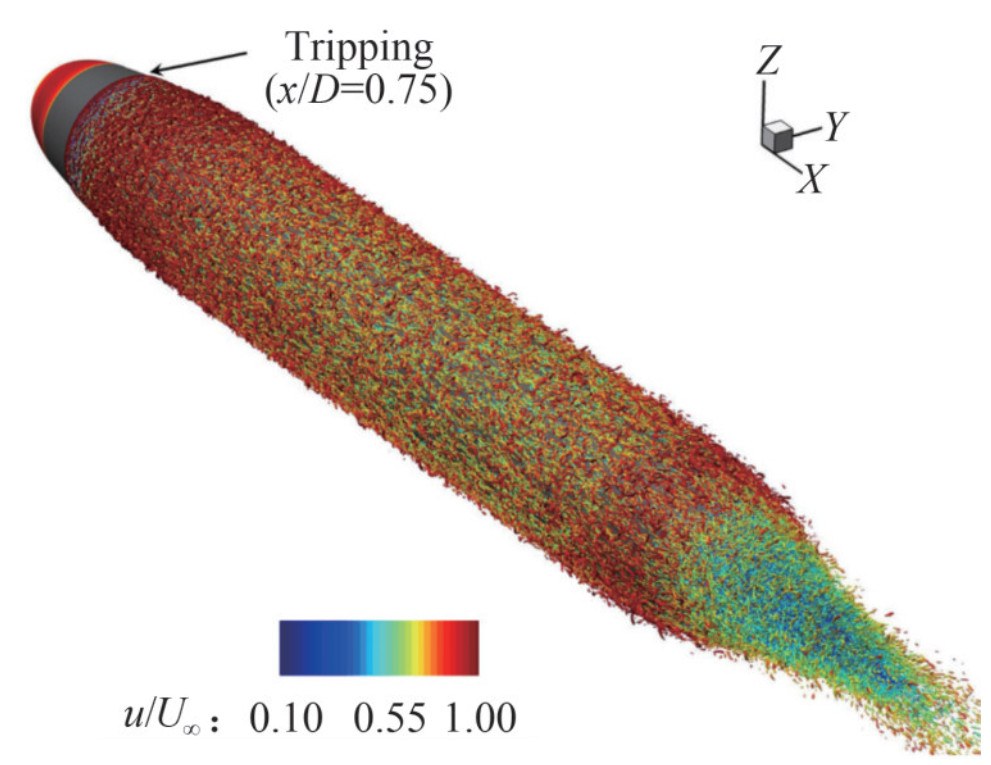Figure  21  Instantaneous flow structures near the wall visualized using the Q-criterion isosurface (Liu et al., 2023)

Download: Full-Size Img

4   Flow over the stern and wake

4.1   Adverse pressure gradient turbulent boundary layer

For the flow over the stern, the tapering geometry at the stern causes the incoming boundary layer to experience strong streamwise pressure gradients and changes the velocity profiles in the boundary layer. As the flow develops, flow separation may occur because of viscous effects and an increase in the adverse pressure gradient. Typical velocity profiles at representative locations along the surface are shown in Figure 22. At the separation location (profile A), the velocity gradient at the wall and the wall shear stress are zero. Beyond this location (from B to C), reverse flow occurs in the boundary layer. Because of the boundary layer separation, the average pressure at the stern is considerably lower than that at the forebody, resulting in a large pressure drag. Boundary layer thickness will substantially increase, and an extra turbulent strain rate will be induced (Morse and Mahesh, 2021).

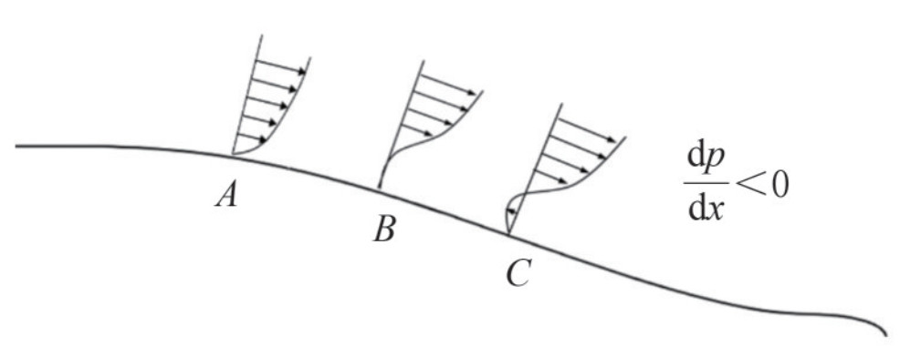Figure  22  Adverse pressure gradient turbulent boundary layer

Download: Full-Size Img

Two parameters have been proposed to describe the strength and history of the pressure gradient, which are generally based on Clauser's parameter β_RC and the shape factor H,

where δ^* and θ are the displacement thickness and momentum thickness of the boundary layer, respectively.

The existence of an adverse pressure gradient causes a fundamental change in the turbulence structure, which increases the difficulty of capture (Krogstad and Skåre, 1995; Schatzman and Thomas, 2017; Kitsios et al., 2017). The flow fulfills unsteady and unstable dynamic interactions and develops inflectional mean velocity profiles in the outer region, which leads to a secondary peak in turbulence production and transfer. Analyzing the velocity structure under specific conditions revealed that sweep motions predominantly occurred slightly above the inflection point, whereas ejections were more prominent below it. In addition, the mean flow in the outer regions of this fully attached boundary layer is characterized by coherent spanwise-oriented vorticity centered around the inflection point.

4.2   Evolution toward self-similarity in the wake

For any wake-generating body, the mean flow is anticipated to exhibit the self-similarity when a substantial distance downstream is considered (Townsend, 1956). The wake of the underwater vehicle, as shown in Figure 23, can be characterized by the maximum velocity deficit, u₀, and half-wake width, l₀. Typically, u₀ and l₀ evolve following the power law scaling relationships expected from the similarity arguments. For an axially symmetric wake, u₀ and l₀ satisfy

Figure  23  Evolution toward self-similarity in the wake

Download: Full-Size Img

where x₀ is the virtual origin of the self-similar wake.

4.3   Numerical simulation methods

RANS encounters challenges because a considerable portion of the physics is embedded in semiempirical turbulence models, leading to outcomes that may prove challenging to validate for accuracy (Alin et al., 2010). Predicting the flow over the stern and wake using RANS is difficult because of the unsteady dynamic interactions in the boundary layer, adverse pressure gradient, shear layer, and junction flow (Posa and Balaras, 2016). Therefore, most studies focusing on the flow around the stern and wake have adopted the LES method or the hybrid RANS/LES method.

4.3.1   LES method

Posa and Balaras (2016) performed a numerical simulation of the near-wall flow over the stern and wake of a DARPA SUBOFF body with appendages at Re_L=1.2×10⁶. Their results confirmed that the wake of the body is influenced mainly by the shear layer from the trailing edge of the fins and the TBL growing along the stern. The complexity of the stern flow is analyzed, and the source of the bimodal behavior of the turbulent stresses in the wake is traced back to the thick boundary layer over the stern. The self-similarity of wake evolution about maximum velocity defect and half-wake width is also investigated up to nine diameters downstream of the tail, as shown in Figure 24. The nine downstream locations are at increasing distances from the tail, with a step equal to the maximum hull diameter.

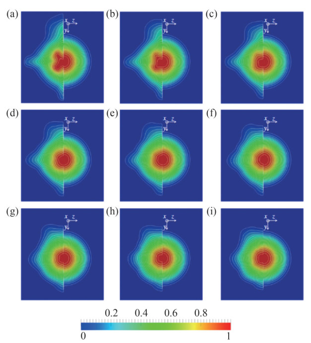Figure  24  Time-averaged fields of the velocity defect in similarity coordinates in the wake of the DSub (Posa and Balaras, 2016). Posa's numerical solution is shown on the left, whereas the self-similar axial symmetric solution proposed by Jiménez et al. (2010b) is shown on the right

Download: Full-Size Img

Kumar and Mahesh (2018a) presented a numerical analysis of near-wall flow structures and wake evolution on the bare hull DARPA SUBOFF model at Re_L=1.1×10⁶ using WRLES, as shown in Figures 25 and 26. A good agreement with the experiments was obtained. The mean streamwise velocity exhibited the self-similarity in the wake, whereas the turbulent intensities were not self-similar over the length of the simulated wake. A thickening of the hull boundary layer due to the adverse pressure gradient on the stern was observed, which eventually led to flow separation and wake formation. The axisymmetric wake was first observed to shift from high-Re to low-Re equilibrium self-similar solutions.

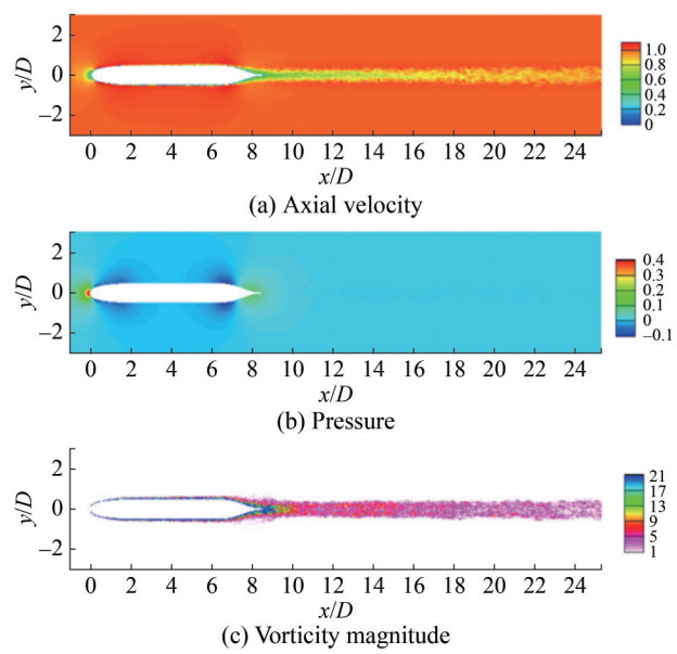Figure  25  Contours of instantaneous flow field in the xy plane (Kumar and Mahesh, 2018a)

Download: Full-Size Img

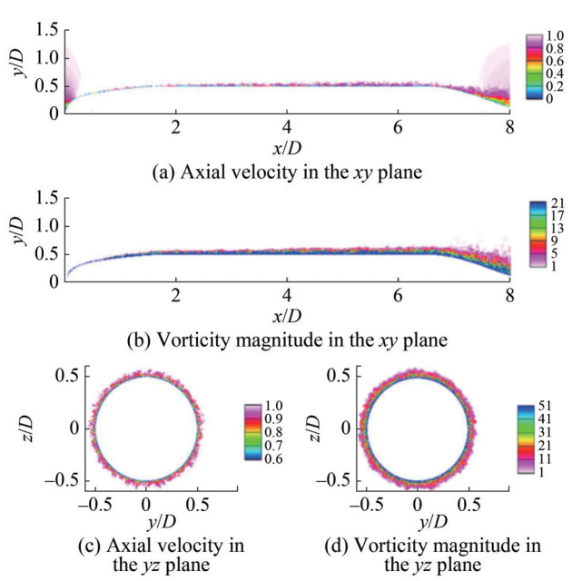Figure  26  Hull boundary layer: instantaneous axial velocity and vorticity magnitude in the xy and yz planes (Kumar and Mahesh, 2018a)

Download: Full-Size Img

To investigate the effects of Reynolds numbers on the flow structure over the stern, Posa and Balaras (2020) extended WRLES to resolve the turbulent flows near the stern of flows around DARPA SUBOFF with appendages at Re_L=1.2×10⁷ and Re_L=1.2×10⁶. Their research revealed that the adverse pressure gradient substantially influenced the TBL over the stern, nearly irrespective of the Reynolds number. They observed that under higher Reynolds number conditions, a less pronounced peak in TKE emerged in the outer layer over the stern. In the study by Zhou et al. (2020), WRLES and WMLES were employed to analyze an axisymmetric body of revolution. This investigation focused on a detailed analysis of the space–time characteristics of velocity and pressure fluctuations within the boundary layer of the tail cone. The predicted velocity statistics exhibited strong agreement with the experimental results, suggesting that the development of the TBL in the tail cone was not considerably influenced by the upstream near-wall structures. Morse and Mahesh (2021) presented a novel approach for analyzing TBL on the stern. They observed that the boundary layer near the stern initiates with a thickness slightly exceeding 20% of the local hull radius and rapidly expands to more than six times the local radius as it reaches the end of the stern. They found that the effect of streamwise curvature created additional streamline-normal pressure gradients such that the pressure varied substantially across the boundary layer, as observed by Patel et al. (1974), Morse and Mahesh (2021).

Chen et al. (2023) investigated the flow around the DARPA SUBOFF model at Re_L=1.2×10⁷ using WMLES. The thickening of the TBL around the stern and the expansion of the wake can be clearly observed through flow using the Liutex vortex identification method, as shown in Figures 27 and 28. To assess the effectiveness of WMLES in turbulent flows near walls, the impact of different wall stress models and sampling distances were also assessed.

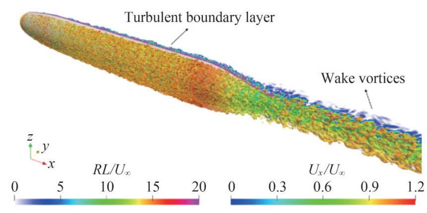Figure  27  Instantaneous vortical structures using the isosurface of $\tilde{\varOmega}_R$=0.52 with the symmetry plane y/D=0 showing the Liutex magnitude (Chen et al., 2023)

Download: Full-Size Img

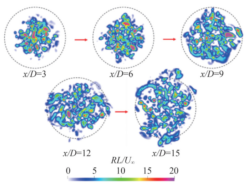Figure  28  Instantaneous Liutex magnitude at different streamwise locations in the wake (Chen et al., 2023)

Download: Full-Size Img

Notably, the wake generated by the propeller will interact with the wake generated by the stern if the propeller is arranged after the stern. Norrison et al. (2017) used the WMLES method to study the flow around a full-scale, fully appended Joubert generic submarine. The propeller model was the DSTG 057–1 propeller, which was a right-handed, generic seven-bladed submarine propeller. The interaction between the wake generated by the propeller and that generated by the stern was discussed. Figure 29 shows vortical and wake structures visualized with isosurfaces of λ₂= − 0.05 (Jeong and Hussain, 1995), and Figure 30 illustrates local flow structures around the rudders and in the propeller near the wake. The tip vortices were found to shed from the propeller blades, and a central and hub vortex was formed and extended downstream of the wake generated by the stern. They also showed the axial velocity distribution on the meridian plane, as shown in Figure 31. The wake was strongly influenced by the propeller, and the nonuniformity of the velocity field due to the presence of the propeller was clearly observed.

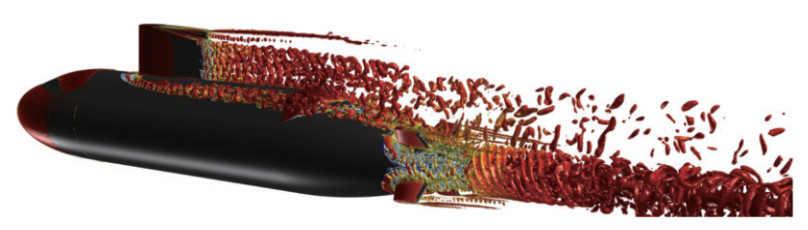Figure  29  Vortical and wake structures (Norrison et al., 2017) visualized with isosurfaces of λ₂=−0.05 (Jeong and Hussain, 1995)

Download: Full-Size Img

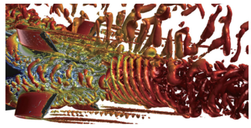Figure  30  Flow structures around the rudders and in the propeller near the wake (Norrison et al., 2017)

Download: Full-Size Img

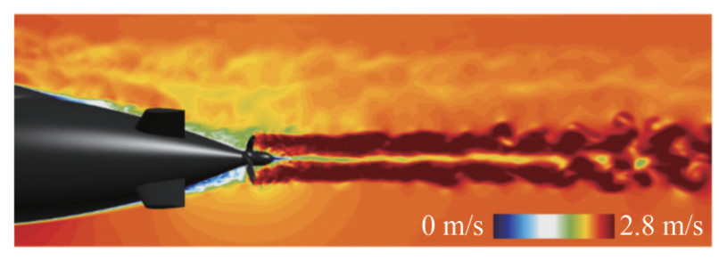Figure  31  Contours of instantaneous axial velocity on the centerline plane in the wake region (Norrison et al., 2017)

Download: Full-Size Img

4.3.2   Hybrid RANS/LES method

LES is expensive because of the TBL at high Reynolds numbers. Massive computing costs are required, particularly for ship hydrodynamics, because they involve high Reynolds numbers on the order of 10⁶ at the model scale and 10⁹ at the full scale, and the flow is characterized by a wide spectrum of turbulent scales. The hybrid RANS/LES approach is an alternative method with high efficiency and acceptable accuracy for turbulent flows at high Reynolds numbers.

The detached eddy simulation (DES) proposed by Spalart et al. (1997) is the most famous hybrid RANS/LES approach that treats boundary layers using a RANS model and applies LES to separated regions. This approach reduces computing costs compared with WRLES while retaining many of the unsteady features of the flows. Some shortcomings were reported in the hybrid RANS/LES approach, such as erroneous activities of the near-wall damping terms in the LES branch, incursion of the LES branch inside the boundary layer, gray area, and log-layer mismatch. However, these shortcomings have been addressed or alleviated in later revisions, such as delayed DES (DDES) (Spalart et al., 2006), improved DDES (IDDES) (Shur et al., 2008), and extended DDES (Patel and Zha, 2020). He et al. (2017) and He and Liu (2018) developed a dynamic DDES model based on the SST k − ω model, in which the log-layer mismatch problem is alleviated by dynamically computing the model coefficients. Alin et al. (2010) conducted a comprehensive investigation of the current capabilities of DES and LES for underwater vehicles, in which the k − ω -based DES appears to somewhat overpredict the magnitude of the velocity fluctuations. We presume that such overpredictions may be due to the eddy viscosity assumption of the RANS method.

Bhushan et al. (2013) evaluated hybrid RANS/LES models to predict the flow around DARPA SUBOFF geometries. The results showed that the influence of the turbulence model on the prediction of surface pressure was almost negligible, whereas the prediction of surface friction strongly depended on the wall function formula. Liu et al. (2021) used a hybrid RANS/LES approach to investigate turbulent flow around a bare DARPA SUBOFF model at Re_L=1.2×10⁶. This hybrid RANS/LES approach employed afull Reynolds stress model (RSM) in the RANS branch to consider the Reynolds stress anisotropy, streamline curvature, and flow separations in the boundary layer. The study compared time-averaged surface pressure coefficient distribution, friction coefficient distribution, and velocity statistics with experimental data (Huang et al., 1992) and WRLES results (Posa and Balaras, 2016), demonstrating a good agreement. The wake flow structures are visualized using the isosurface of the instantaneous Q-criterion, as shown in Figure 32. The instantaneous contours of the TKE overlap the projection of streamlines at the stern, as shown in Figure 33. Large-scale turbulent motions around the stern were successfully captured. The RSM-based hybrid RANS/LES approach effectively captured separated flow with surface curvature, adverse pressure gradient-induced separation, and strong interactions among various stresses, providing improved predictions of unstable flow near the tail.

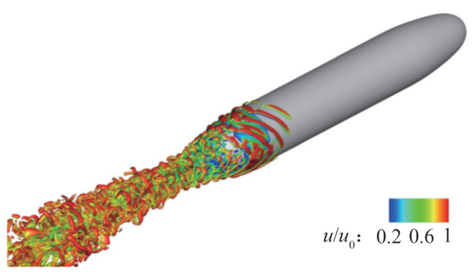Figure  32  Wake flow structures are visualized using the isosurface of the instantaneous Q-criterion with the RSM-based hybrid RANS/ LES approach (Liu et al., 2021)

Download: Full-Size Img

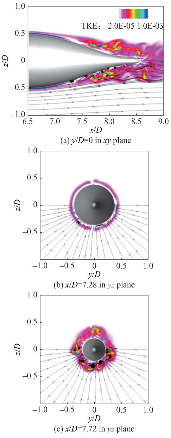Figure  33  Contours of TKE overlapping with the projection of streamlines obtained by RSM-based IDDES (Liu et al., 2021)

Download: Full-Size Img

5   Flow around the appendages

5.1   Complex turbulent vortex structures

Appendages such as sails, rudders, and fins are set in an underwater vehicle to meet practical needs and maintain balance and stability. The presence of appendages will directly lead to the sudden geometric deformation, which induces increasing drag and complex vortex structures as well as an unsteady wake aft of the appendages (Alin et al., 2010). The sudden geometric deformation will also complicate numerical simulation because of the difficulty in mesh generation around the appendages.

Turbulent vortex structures around appendages can be mainly divided into three types according to their shape: 1) horseshoe vortex, 2) necklace vortex, and 3) hairpin vortex (Qu et al., 2021). The horseshoe vortex has a high-intensity U-type structure and is generated at the junction of the sail and hull. The hairpin vortex is formed and observed in the downstream direction with high and extremely unsteady velocity as the horseshoe vortex develops. The necklace vortex has a necklace structure and is formed by the rotation of the boundary layer at the edge of the sail. It is shed at the top of the sail and developed along the flow direction.

5.2   LES with the immersion boundary method

Because of its thorough resolution of vortices and precise treatment of turbulent flow details, LES has been widely applied to study underwater vehicles with appendages. Otherwise, the immersion boundary method (IBM) is also applied to solve the flow around the complex geometry of appendages because of the advantage of dealing with wall boundaries. Wang et al. (2016a) used WMLES with IBM based on moving least-squares reconstruction to simulate the complex flow around the DARPA SUBOFF with full appendages. They observed that the flow originated from the top of the sail and progressed downstream as a tip vortex. This tip vortex subsequently interacted with the boundary layer in the midbody region. Fureby et al. (2016) used WRLES and captured the detailed turbulent structures around the fully appended DSTO generic submarine model under straight ahead conditions and during a 10° side-slip. They found that the flow over the sail was dominated by two sets of vortex structures. The primary set of vortices originated from the widest section of the sail, extending substantially rearward and positioned well above the stern rudders. Simultaneously, a secondary pair of vortices were formed directly from the leading edge of the sail. These vortices ascended above the main vortex pair and subsequently descended along the trailing edges of the sail, dividing the wake into two distinct sections. As the horseshoe-vortex system developed, the interaction between vortex instabilities and the hull boundary layer caused the leg fragmentation of the horseshoe-vortex system. Consequently, connected vortex loops began to form. Posa and Balaras (2020) studied the effects of Reynolds number on the flow around the fully appended DARPA SUBOFF at Re_L=1.2× 10⁶ and 1.2×10⁷. IBM was used to reconstruct the velocity near the body. WMLES was applied to simulate the turbulent flow on the midbody, whereas WRLES was applied on the stem and wave region. They used the Q-criterion to identify the vortex structure and found that the vortex formed at the leading edge of the stern appendages generated secondary vortices in closer azimuthal positions, eventually evolving into primary vortices downstream. Concurrently, these vortices were intensified at the trailing edge of the fins, where maximum circulation values were observed at both Reynolds numbers. Notably, the junction vortices exhibited greater strength at higher Reynolds numbers, correlating with higher circulation values.

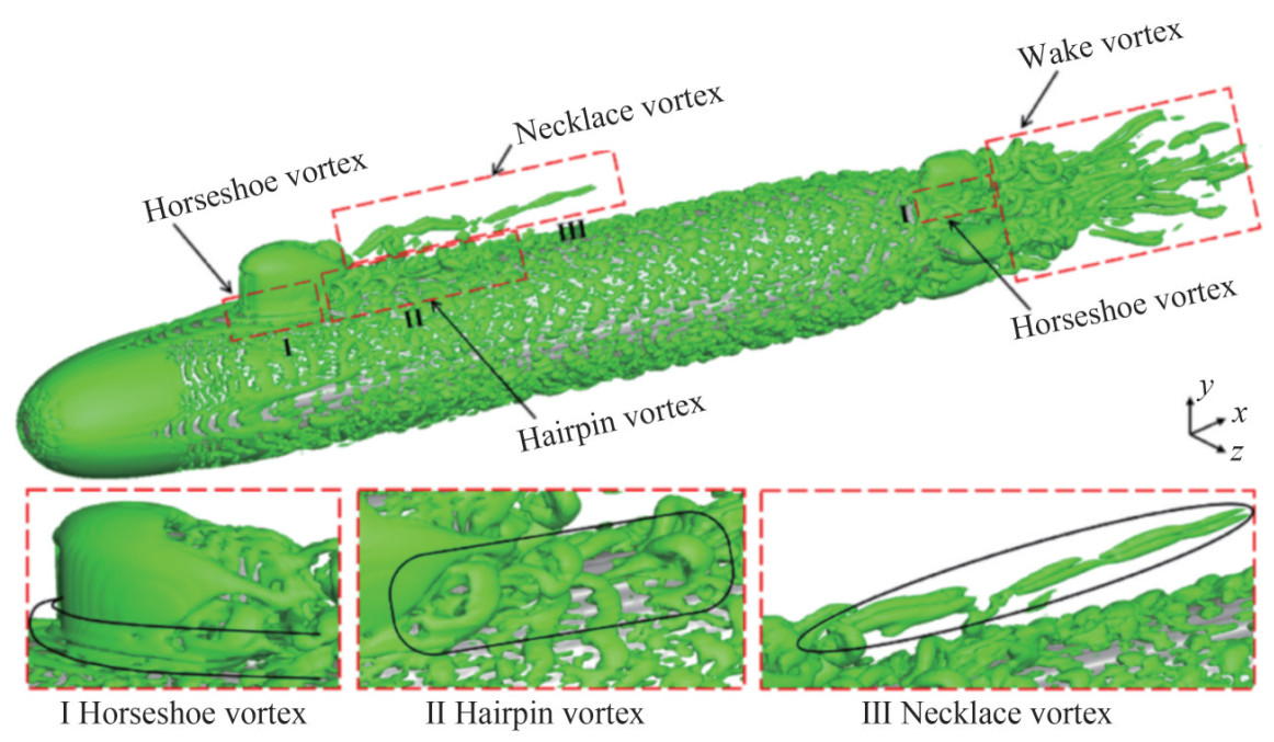Figure  34  Vortex structures around the DARPA SUBOFF at Re_L = 1.2 × 10⁷ (Qu et al., 2021)

Download: Full-Size Img

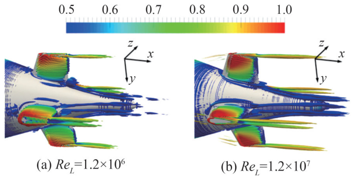Figure  35  Vortex structures at the leading edge of the stern appendages at Re_L=1.2×10⁶ and Re_L=1.2×10⁷ (Posa and Balaras, 2020)

Download: Full-Size Img

Qu et al. (2021) used WMLES with the boundary data immersion method to simulate the complex flow around the DARPA SUBOFF with full appendages. They used the Q-criterion (Hunt et al., 1988) and the Liutex method (Liu et al., 2018; Liu et al., 2019a, b) to identify and analyze the vortex structures behind the sail and discussed the formation mechanism of turbulent vortex structures around the appendages. The horseshoe vortex behind the sail, as shown in Figure 36, was primarily generated by the substantial adverse pressure gradient at the leading edge of the sail and the lateral acceleration along the sides of the sail. The evolution of the hairpin vortex, as illustrated in Figure 37, involved the dissipation of the vortex leg, distortion of the O-type structure, and subsequent transformation into a U-shaped structure. The development of the necklace vortex involves extension, distortion, fracture, and subsequent division into two parts, as shown in Figure 38. Meanwhile, they found that the horseshoe vortex played a dominant role in turbulence structures and that rotation was dominant in the vortex distribution profile. Zhou et al. (2022) used WRLES with IBM to simulate turbulent flow around the fully appended DARPA SUBOFF at Re_L=1.2×10⁷. The results showed that the effect of the sail-tip vortex on turbulent flow was limited to a local region on the upper surface of the midbody. Rocca et al. (2022) applied WMLES to simulate the turbulent flow around the fully appended BB2 submarine at Re_L=1.2×10⁶. They captured the sail-tip, fin-tip, junction, and horseshoe vortices around the appendages, as shown in Figure 39. They also found that the sail on the upper side of the hull generated an adverse pressure gradient that determined the formation of a horseshoe vortex (Qu et al., 2021).

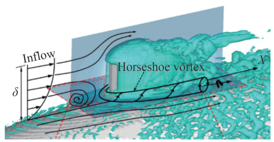Figure  36  Horseshoe vortex behind the sail (Qu et al., 2021)

Download: Full-Size Img

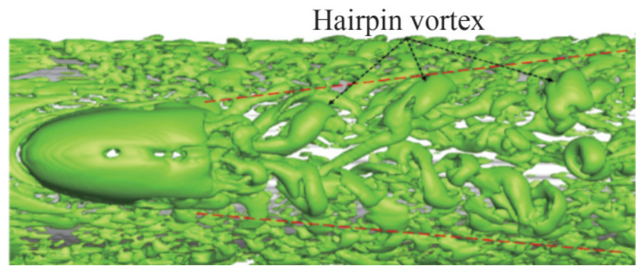Figure  37  Hairpin vortex behind the sail (Qu et al., 2021)

Download: Full-Size Img

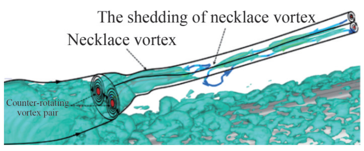Figure  38  Necklace vortex behind the sail (Qu et al., 2021)

Download: Full-Size Img

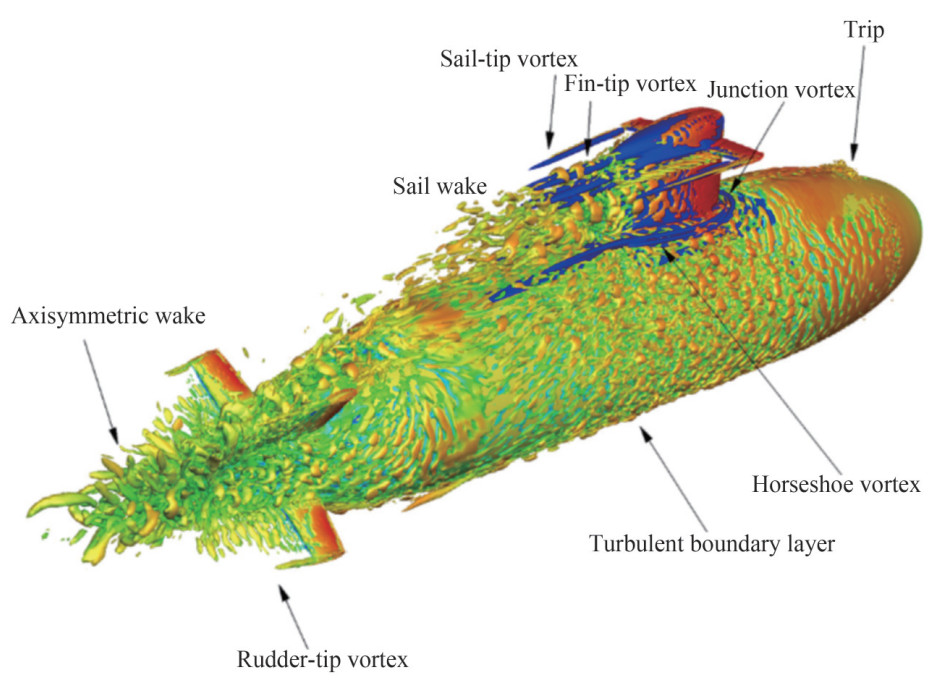Figure  39  Turbulent structures around the BB2 submarine at Re_L=1.2×10⁶ (Rocca et al., 2022)

Download: Full-Size Img

6   Conclusions and future perspectives

This paper introduced the typical geometric features of underwater vehicles, resulting in distinctive flow structures at various positions on these vehicles. The summarized flow structures at different locations, namely, the forebody, midbody, stern, and appendages, encompass aspects such as transition, turbulent flow, curvature effects, pressure gradients, wakes, and complex vortex structures. The review also addressed the current issues and challenges associated with capturing these flow structures. Furthermore, it provides an overview of suitable computational methods for effectively capturing focal flow structures. This comprehensive review is a valuable reference for examining flow and noise phenomena in the context of underwater vehicles.

In the future, numerical simulation will be still the main method for studying the turbulent flow around underwater vehicles because of its great advantages. High-precision, low-dissipation, and high-resolution numerical simulation methods are the trend for meeting the requirements of studying mechanisms and predicting noise. Higher computational performance and efficient parallel algorithms are also required to capture precise flow structures.