1   Introduction

Much scientific and engineering interest has been directed towards understanding exceptionally large waves with relatively low probabilities of occurrence in view of their potentially destructive effect on ships (Guedes Soares et al. 2008; Fedele et al. 2017) and offshore structures (Fonseca et al. 2010). In this respect, model tests in a laboratory have demonstrated their usefulness and reliability for studying rare nonlinear wave phenomena and the responses of marine structures to them.

Abnormal waves have been often attributed to higher-order mechanisms among which is the Benjamin-Feir modulational instability resulting from third-order quasi-resonant interactions between free wave modes (Dysthe et al. 2008). Indeed, nonlinear focusing can explain some of the reported large discrepancies from linear and second-order wave models in long-crested seas (Fedele et al. 2010; Shemer and Sergeeva 2009; Cherneva et al. 2013). Over the years, attention has been paid to this mechanism by studying the evolution of wave envelopes (Onorato et al. 2001; Janssen 2003; Zhang et al. 2015a; among others) and the ratio between wave steepness and spectral width, known as the Benjamin-Feir index, has been proposed to quantify the tendency for evolving extremes due to quasi-resonance under certain unidirectional conditions (Janssen 2003). It has been also found that the coefficient of kurtosis of narrowband unidirectional seas simply depends on the squared BFI (Mori and Janssen 2006). This dependence stands for the large-time asymptote of the so-called dynamic component of the coefficient of kurtosis resulting from third-order quasi-resonant wave-wave interactions. There is also the bound wave contribution to the kurtosis induced by both second- (Tayfun 1990; Fedele and Tayfun 2009) and third-order bound nonlinearities (Janssen and Bidlot 2009). The BFI has been further generalized by Janssen and Bidlot (2009) to include more realistic effects, such as directional spreading, characteristic of the oceanic wave fields. A summary of the evolutionary properties of mechanically generated 2D and 3D waves triggered by nonlinear focusing, as well as the adequacy of some nonlinear deterministic wave models to capture higher-order effects can be found in Zhang et al. (2019).

A wave train becomes unstable towards long-crested conditions due to the possibility of interaction between freely propagating elementary waves (Janssen 2003; Fedele et al. 2010). Narrowband long-crested waves have been systematically reproduced in wave flumes and offshore basins, and the properties of the generated wave fields studied statistically (Onorato et al. 2004; Waseda et al. 2009; Shemer and Sergeeva 2009). Such random wave fields have been also numerically simulated using deterministic nonlinear models to predict their evolution (Socquet-Juglard et al. 2005; Slunyaev et al. 2005, 2014; Toffoli et al. 2008; Zhang et al. 2015b, 2017). However, both controlled experiments and numerical simulations, although providing insight into the phenomenon of abnormal waves, have been questioned regarding how realistic their predictions are, considering that the oceanic extremes commonly originate from wave fields with relatively broad spectra in terms of frequency and directional spreading (Forristall 2007; Guedes Soares et al. 2011).

This controversy increases further if one considers that the oceanic waves are forced by the wind and have random structure, as discussed by Fedele et al. (2016). While the instability process cannot be the primary reason for extreme wave formation, cases of heavy conditions at sea related to accidents and worsened operability of ships and offshore platforms are explained by coexisting crossing wave systems (Cavaleri et al. 2012). Another plausible explanation for the wave extremes at sea is the linear focusing of elementary waves enhanced by second-order bound modes which agree with field measurements (e. g. Tayfun 2008; Tayfun and Fedele 2007). Theoretically, investigations on the adequate statistical and probabilistic description of nonlinear wave fields were originated by Longuet-Higgins (1963) for second-order random waves. For many years, the second-order approximation has been considered the most elaborated theory for design, as far as the statistical models of wave crests and troughs have been able to provide a reasonable fit to field measurements (Forristall 2000; Petrova et al. 2006; Tayfun 2006; Fedele and Tayfun 2009). Comparative studies of abnormal waves at sea, however, have demonstrated that the wave extremes remain significantly underestimated by the standard models (Stansberg 2000; Guedes Soares et al. 2003, 2004a, 2004b; Petrova et al. 2007; Cherneva and Guedes Soares 2008). Crest extremes in high sea states from offshore basins showed also to be slightly underpredicted by the second-order model which has been attributed to higher-order effects in unidirectional waves (Stansberg 2001; Petrova and Guedes Soares 2008).

To improve the statistical predictions, formulations based on the Gram-Charlier or Edgeworth series expansions have been proposed (Janssen 2003; Tayfun 2006; Mori and Janssen 2006; Tayfun and Fedele 2007), where the nonlinear effects are captured through higher-order moments of the elevation process. While these models have been found unable to describe significant non-Gaussian behaviour in oceanic data, they are effective in wave flumes and numerical 2D simulations (Petrova et al. 2013; Cherneva et al. 2013; Shemer and Sergeeva 2009). This is to be expected, as far as the approximations are based on the narrowband assumption which reduces their applicability to extreme events in controlled environments, such as wave flumes and numerical simulations.

The various theories and models discussed describe different properties of extreme sea states and abnormal waves, but they all need validation with physical data, which is extremely important. Ocean measurements provide data in the real environment but they are obtained very seldomly and often there is no additional information on the background conditions that generated the measured records. Attention is then addressed to laboratory data, which can have the generation and other boundary conditions known and controlled. However, the characteristics of the generated waves have differences from the ocean environment as the input wind energy is not present in the wave fields and the boundaries of the tanks provide artificial conditions not existing in the ocean. At any rate, the observation of the wave propagation along the tanks and the analysis of how the nonlinearities develop has brought an important understanding of the phenomena.

There are not many systematic studies performed in this field as the various facilities are more focused on reproducing the wave conditions at the central location of the tank where they will place the structures to be tested. Knowledge of how waves propagate along the tanks has had less attention and this will be influenced by the specific features of each facility. An experimental program was conducted at MARINTEK ocean basin in 1999, leading to several studies such as Petrova and Guedes Soares(2008, 2009), Cherneva et al.(2009, 2013), Fedele et al. (2010), Zhang et al.(2014a, 2015b). About 10 years later a new study was made at MARINTEK with a similar arrangement but expanding the scope to consider directional aspects, again leading to several studies such as Onorato et al. (2009), Toffoli et al. (2010), Zhang et al. (2016). Other studies made at the Ocean Basin of the Danish Hydraulic Laboratory also produced useful results (Petrova et al. 2011).

Similar studies have been also made in wave towing tanks where the influence of the lateral boundaries is larger and this was reflected in the analysis produced for the data of the tank of the Technical University of Berlin (Cherneva and Guedes Soares 2011) and the one from the El Pardo Hydrodynamic Laboratories in Madrid (Zhang et al. 2013, 2014a).

This paper presents the results of a similar type of study now conducted at the Brazilian Laboratory for Ocean Technology, as the first experimental study of this kind was conducted in that laboratory. Therefore, the importance of this study is that it allows confidence to be established on the ability to make studies of this kind in that facility and it provides benchmarking with earlier studies as some of the sea states analysed are the same that have been tested earlier in other facilities.

The present paper shows results on the non-Gaussian statistical properties of laboratory-generated unidirectional deep-water random wave fields characterized by JONSWAP spectrum. In particular, the study aims at assessing the importance of third-order nonlinearity on wave statistics in the presence of large waves defined as abnormal by some existing criteria. The behaviour of statistical quantities indicating increased probability for large amplitude events is considered in view of existing favourable conditions for the development of Benjamin-Feir instability. These conditions are formally quantified by the Benjamin-Feir index. The propagated distance, on the other hand, reflects the stage of evolution of the instability, thus of the wave field nonlinearity.

The structure of the paper is as follows. Section 2 describes the ocean basin facility and the experimental set-up, as well as gives the basic properties of the generated wave fields. Section 3 provides an analysis of the observed characteristic statistical and spectral sea state parameters and shows the dependencies between them against existing theoretical and empirical models. Also, the spatial variation of these parameters is demonstrated and discussed in view of developing nonlinear instability. Section 4 focuses on the largest wave crests and crest-to-trough wave heights and addresses the effect of breaking on the measured extremes. A summary of the conclusions is presented in Section 5.

2   Laboratory conditions and experimental set-up

The wave data used to perform the study represent measurements of the free surface fluctuations about the mean water level. They were collected during an experiment carried out in the Brazilian Laboratory for Ocean Technology (LabOceano, Brasil) in 2017.

Figures 1(a) and (b) illustrate the ocean basin with dimensions: 40 m length, 30 m width and 15 m depth, except for the central pit with an additional 10 m depth. The movable basin floor can be adjusted so that the water depth can vary between 2 m and 14.6 m. In the actual laboratory experiment, the bottom was at depth of 14.6 m. The basin is supplied at the short side with a multi-flap wavemaker consisting of 75 individually controlled flaps for the generation of short-crested and long-crested waves (Figure 1(a)).

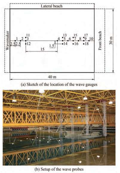Figure  1  Sketch of the offshore basin facility of LabOceano and the test equipment

Download: Full-Size Img

The wave reflections have been measured in an earlier experiment with regular waves and summarized in an internal report. Following the algorithm of Mansard and Funke (1980), the reflection coefficients have been calculated between 3.9% and 16.6% depending on the wave height and period. The problem with the reflection and wave build-up has been resolved by means of two parabolic wave absorption beaches of wooden panels; the beach in front of the wavemaker is 8 m wide and the lateral beach has a width of 5 m.

Random wave fields have been generated using the JONSWAP formulation as an input to the wavemaker (Hasselmann et al. 1973; Komen et al. 1994)

where σ₀ is the spectral width parameter: σ₀ = 0.07 for ω < ω_p, and σ₀ = 0.09 for ω ≥ ω_p; g is the gravity acceleration; γ is the peak enhancement factor; α is the Phillips constant – a scaling parameter used to adjust the spectral energy to the desired significant wave height and ω_p (rad/s) is the angular peak frequency. Each free surface realization uses as an input randomly chosen amplitudes and phases.

The conducted laboratory experiment resulted in 90 irregular long-crested sea surface realizations which represent a combination of 9 sea state steepnesses with 2 peak enhancement factors (γ = 3 and 6) and 5 seeds for each pair initial steepness – γ. Eventually, combinations for 3 cases of steepness, designated as tests 1 to 6 in Table 1, were chosen for analysis.

Table 1 specifies the input wave conditions at the wavemaker in a model scale 1:1 which allows to convert directly to any prototype scale. The JONSWAP frequency spectra are defined in terms of the following parameters: significant wave height H_s = 4σ, where σ = m₀^1/2 stands for the standard deviation of the free surface elevation expressed from the zeroth spectral moment; peak period T_p = 1 s; peakedness parameter γ; Phillips constant α and steepness parameter ε = k_p H_s /2 – a measure of nonlinearity, where k_p is the wave number associated with T_p. The parameter Δω represents the spectral width around the peak and is estimated as half-width at half of the spectral maximum so that the relative bandwidth Δω/ω_p is a measure of wave dispersion. The last column of Table 1 shows the values of the Benjamin-Feir index calculated from the definition of Janssen (2003)

Onorato et al. (2004) provided the first experimental evidence that the BFI can influence significantly the large wave statistics and thus the probability of rogue wave occurrence in the time series. In particular, a random wave train becomes unstable when BFI > 1. Table 1 shows that this condition is fulfilled for the experimental runs with moderate and large wave steepness, ε = 0.141 and ε = 0.181.

As can be seen in Table 1, the prescribed steepnesses at the wavemaker are the same for each pair, however, the input spectra with γ = 6 are narrower, due to the added peaked energy, as compared to γ = 3 (Figure 2). Consequently, larger values of γ imply a larger Benjamin-Feir index which shows a more probable occurrence of unstable conditions due to quasi-resonance around the spectral peak followed by an increase of the wave nonlinearity. The Phillips constant α is also related to the wave steepness as α ~ ε², since it is a scaling factor for the energy of the wave field. For example, Onorato et al. (2001) argue that by making α double for fixed γ, the steepness increases by a factor of √2 and so does the BFI.

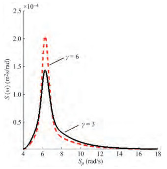Figure  2  JONSWAP spectrum with H_s = 0.07 m and T_p = 1 s

Download: Full-Size Img

The instantaneous surface elevations around the mean water level were simultaneously measured by conductive-type wave gauges based on the Danish Hydraulic Institute (DHI) wave probe system. These wave gauges have a behaviour similar to other commercial wave gauges and thus no specific study was made for their calibration as they have been calibrated by the Ocean Basin before being routinely used. They were deployed at 18 locations in the tank (Figure 1(a)). However, the analysis here concentrates only on the recordings from the 10 gauges aligned with the central axis of the basin. The probes are located at a uniform distance of 2.5 m; the nearest gauge is placed at 2.5 m away from the wavemaker and the distance between gauge 3 and gauge 4 is 15 m.

Furthermore, a preliminary comparison of the wave records from the sets of three probes at a constant distance along the basin (Figure 1) has shown consistency between the measurements in terms of registered spectral energy. The total duration of each experimental realization is 20 min in model scale with a sampling step dt = 0.016 7 s. The wave-by-wave analysis resulted in approximately 1 200 waves when using either of the zero-crossing wave definitions or a total of 6 000 for the ensemble of five experimental realizations for each spectral condition at the wavemaker (Table 1). The larger number of sampled waves reduces the statistical uncertainty when estimating higher-order statistics and allows for achieving convergence at the tails of the probabilistic distributions. For each experimental run, the transient effects of the start-up have been considered by truncating a number of ordinates at the beginning of the time series. The initial truncation depends on the location of the gauges and the group velocity of the second harmonic of the spectral peak, c_g = 0.39 m/s, which define the time necessary for the associated energy group to travel the distance to the wave gauge. Each record has been also corrected for the mean water level, resulting in a zero-mean wave process.

It must be noted here that all results and comparisons presented next are in model scale.

3   Laboratory data: basic spectral and statistical parameters

The experiments were designed to obtain irregular waves propagating on deep water of constant depth, d = 14.6 m. The deep-water conditions are verified by the relative water depth, d/L_p. Thus, for T_p = 1 s, the linear dispersion relationship gives d/L_p = 9.36, where the length of the peak frequency harmonic is calculated as L_p = gT_p²/(2π) = 1.56 m.

The relative water depth in terms of k_pd, on the other hand, can be used as an indicator for modulational instability since k_pd < 1.36 sets the upper bound of stability against side-band perturbations (Onorato et al. 2006). Consequently, in the present experiment, all sea states provide favourable conditions for the development of large-amplitude events as a result of instability.

The large number of free surface realizations for different initial steepnesses allows not only to obtain more reliable statistics by reducing the statistical variation but also to study in a more consistent way the development of wave nonlinearity along the basin and its effect on some principal statistical and spectral characteristics presented and discussed next. These characteristics have been estimated as ensemble averages over each of five test runs of identical input steepness and spectral peakedness factor.

Figure 3 illustrates the wave field energy in terms of the area under the spectral density curve, m₀, as a function of the propagated distance. As can be seen, the energy remains relatively unchanged along the basin. A general agreement can be seen with the input energies for the moderate and steep sea states (Figure 3(a)) which are illustrated as horizontal lines. An exception from this agreement are the low sea states in Figure 3(b) which are slightly below the reference values. The observed deviations in the spectral energy can be partially attributed to experimental uncertainties associated with the calibration of the wave sensors which are estimated to be between 1 and 2 mm, depending on the wire length.

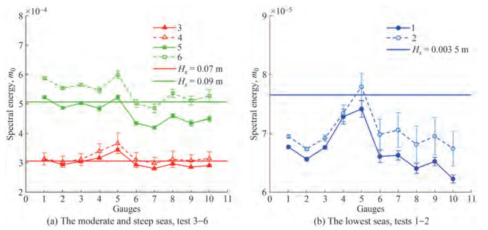Figure  3  Variation of the spectral energy m₀ with the distance. The horizontal lines in the plots illustrate the reference spectral energies

Download: Full-Size Img

Furthermore, the included error bars show the effect of measurement uncertainties. They follow from statistical analysis of the sets of five identical experimental realizations (the same H_s, T_p and γ, but different seeds) to evaluate the standard deviation of m₀ for each wave probe and then find the standard deviation of m₀ and the standard error, σ_m0 /N^1/2, where N = 5. It can be seen that only for the moderate sea states (Figure 3(a)) the variations around the reference values fall largely within the range of measurement uncertainty. To clarify further the observed discrepancies, especially for the low sea states in Figure 3(b), it should be added that the usual corrections to achieve the target spectra were not performed in these particular experiments as this was not required. Moreover, the input values of H_s and T_p were treated as initial reference values rather than as a target.

Irrespective of the uncertainties due to calibration, a general trend has been recorded by the sensors describing an increase of m₀ up to gauge 5 (16L_p) followed by a decrease, which becomes more pronounced for larger steepness and BFI, respectively (Figure 3(a)). A possible explanation for the initial increase can be the fact that although the experimental set-up aimed at generating long-crested irregular waves, some small transversal waves flowing from the corner of the basin (at the left side of the wavemaker) to the centre of the tank, could have increased the energy locally.

Figure 3 shows that for the two highest sea states (5 and 6) the spectral energy is relatively stable (with some statistical variations) until gauge 5 and then it decreases a bit. For the intermediate sea states a tendency for the energy to increase until gauge 5 is present and this becomes more evident for the two lowest sea states. Our interpretation of the situation is that the generated waves need some space (time) to grow until their maximum value which in this tank was designed to be at gauge 5, where the structures are to be placed for testing. After that location, the dissipation effects start becoming more important and the energy is dissipated. This effect is not so evident for the higher sea states because they require more energetic action from the generating paddles and this forces the waves to fully develop earlier.

On the other hand, the systematic decrease of the wave energy over the second half of the basin suggests that when the initial steepness increases, wave breaking takes place and energy is dissipated as a result of it. Recently, Babanin et al. (2007) showed that breaking can be expected only if the mean steepness of the wave field exceeds the value of 0.1. Thus, given the experimental conditions in Table 1, breaking should not be expected in the lowest sea states (ε = 0.07, Figure 3(b)). However, it can happen occasionally in the moderate seas which have steepness slightly higher than the threshold (ε = 0.141) and could affect significantly the wave statistics of the severest sea states, where ε = 0.181 is largely beyond the stated limit (Figure 3(a)).

The position of wave breaking is not at one specific point along the tank but a length along which waves will be breaking. There is some uncertainty involved in the breaking process which implies that some waves will break earlier than others. The interpretation is that after gauge 5 wave breaking occurs and this will partially explain the decrease of energy that is observed after gauge 5.

While the energy of the evolving wave field remains generally constant, the transfer of energy between wave components as a result of higher-order wave-wave interactions makes the spectrum evolve. For example, as a result of modulational instability and associated exchange of energy around the spectral peak, the frequency spectrum may experience broadening and downshift. These effects have been observed in numerical experiments (Janssen 2003; Dysthe et al. 2003) and in laboratory measurements (Onorato et al. 2006; Toffoli et al. 2008; Fedele et al. 2010), including also model tests of coexisting crossing seas (Petrova and Guedes Soares 2014). They can be also identified in the spectra of the time series here, as Figure 4 illustrates.

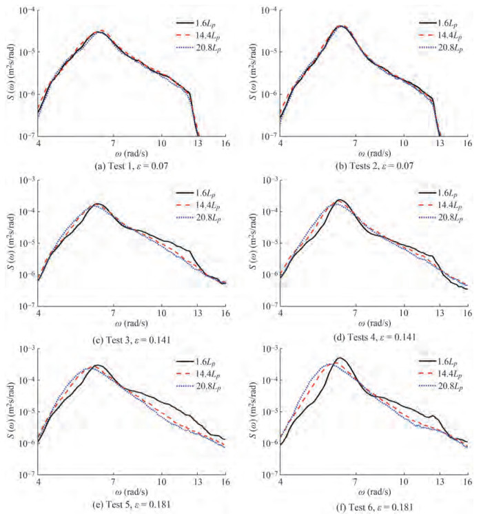Figure  4  Spatial evolution of the wave energy spectrum at three different locations (L_p)

Download: Full-Size Img

In particular, Figure 4 shows in log-log scale the spatial evolution of the ensemble-averaged frequency spectra at three locations along the tank corresponding to different stages of the developing instabilities: weakly-nonlinear waves, intermediate stage and peak stage of development. The propagated distance until the considered gauges is expressed as multiples of the characteristic wavelength L_p: 1.6L_p (gauge 1); 14.4L_p (gauge 4) and 20.8L_p (gauge 8). The set-up of the laboratory experiment allows following the evolution of the wave fields up to approximately 24L_p. The effects of modulational instability, on the other hand, are typically reported after 10 to 30 wavelengths from the wavemaker in sea states with high BFI values (Stansberg 2000; Onorato et al. 2006).

For the low sea states in Figures 4(a) and (b), the spatial changes of the spectral shape and the modal frequency are hardly distinguishable. These spectra are initially the broadest in terms of Δω, as compared to the other sea states, and maintain the broadest over the distance. Pronounced changes, supporting the nonlinear evolution of the unidirectional narrow-banded wave fields, are clearly observed in the moderate sea states (Figures 4(c) and (d)) and especially in the most energetic seas where the BFI reaches 1.702 (Figures 4(e) and (f)). In particular, the broadening of the spectra around the peak reflects increasing instability regions due to the formation of side-band modes. Significant broadening occurs over the first four gauges with the first local peak of ∆ω reached at gauge 4 (14.4L_p); the spectra are depicted in Figures 4(c)–(f) by the dashed red lines. The increase of Δω continues until gauges 7–8 and then stabilizes. The stabilized width spectra for gauge 8 (20.8L_p) are shown as dotted blue lines. In a study of random unidirectional waves with an initially narrow Gaussian spectrum, Shemer and Sergeeva (2009) concluded that the increased nonlinearity is strongly related to the local peaks in the evolution of ∆ω. Thus, the broadening of the initially narrow spectra here could imply a higher probability of encountering extremely large, steep waves.

Figure 4 also allows seeing the variation of the characteristic frequency ω_p along the basin. For the lowest sea states (Figures 4(a) and (b)), it remains nearly unchanged, varying slightly around the mean frequency ω_p = 6.26 rad/s which is close to the frequency at the wavemaker, ω_p = 6.28 rad/s. Unlike the low sea states, downshift can be observed for higher steepness (Figures 4(c)–(f)), where the average frequency of the moderate seas is estimated as ω_p = 6.13 rad/s and of the steepest seas is ω_p = 6.01 rad/s. It must be noted that the first reduction of ω_p occurs only at gauge 4 (14.4L_p). Before that, the modal frequency maintains nearly constant, irrespective of the wave environment at the wavemaker.

The observed peak downshifts and reduction in Figure 4, along with the fact that the wave field energy maintains at approximately the same level with the distance (Figure 3), leads to the conclusion that the steepness of the considered wave fields is generally diminishing. On the other hand, the more efficient downshift of the spectral tail for the sea states with the highest initial steepness (Figures 4(e) and (f)) could imply that the nonlinear effects of quasi-resonant interactions combine with energy loss due to breaking and dissipation. The latter is expected to affect largely the wave and crest maxima and the estimates of the higher-order statistics, in particular the coefficient of kurtosis, as will be shown next.

The self-focusing in unidirectional waves with initially narrow spectra can modify significantly the wave statis tics. Thus, attention is usually paid to statistical quantities indicating increased probability for wave extremes in the wave recordings. Starting from the assumption of weak nonlinearity, the non-Gaussian sea surface is presented as a linear superposition of free wave modes modified by second-order bound harmonics which is visually demonstrated by higher sharper crests and shallower rounded troughs. The introduced vertical asymmetry is statistically expressed by the coefficient of skewness of the surface elevation probability density function, λ₃₀. In particular, the ocean waves have positive skewness, which means a greater probability of large positive displacements than for large negative displacements. Following Tayfun (1994), the third-order normalized cumulant is calculated from the surface elevation, η, and its Hilbert transform, $\hat{\eta}$, as:

On the other hand, the increased frequency of occurrence of large crest-to-trough excursions due to third-order nonlinear wave-wave interactions are indicated by the positive non-zero fourth-order normalized cumulant, λ₄₀ – the coefficient of kurtosis, or by the sum of fourth-order joint cumulants Λ = λ₄₀+3λ₂₂+λ₀₄. These two fourth-order statistics are used as higher-order corrections in the distribution models of wave crests, troughs and heights.

The fourth-order normalized joint cumulants follow the generalized form of Tayfun and Lo (1990)

The magnitude of the coefficient of kurtosis results from the joint contribution of two nonlinear sources: (1) bound wave corrections of order O(ε²) which are negligible for weakly-nonlinear waves; and (2) near-resonant interactions (Benjamin-Feir instability), in a way that for simultaneously narrow spectrum and long-crested waves (2) becomes the dominant factor giving rise to large deviations from the Gaussian statistics (Janssen 2003; Onorato et al. 2005; Mori and Janssen 2006). Moreover, Janssen (2003) showed that, for the particular case of narrow-banded longcrested wave fields at long times, the coefficient of kurtosis strictly relates to the BFI through the quadratic form

The large λ₄₀ commonly indicates an increased frequen‐ cy of occurrence of unusually large waves due to wave grouping (Onorato et al. 2006). On the other hand, large BFI values illustrate that the nonlinearity (steepness) dominates the linear dispersion which leads to higher values of λ₄₀, in agreement with Eq. (5). Consequently, while the BFI could indicate appropriate initial conditions for abnormal waves, λ₄₀ could be taken as a critical parameter reflecting the evolution of nonlinearity and wave extremes in the time series.

The skewness values of the considered surface realizations fulfil the equality applicable for weakly-nonlinear wave process: λ₃₀ = 3λ₁₂, while λ₀₃ ~ λ₂₁ ~ 0 (Tayfun 1994). The joint fourth-order cumulants λ₁₃ and λ₃₁ are essentially zero in this case. It is also expected that λ₀₄ > 3λ₂₂ > λ₄₀, irrespective of the type of spectrum and the angular spread (Tayfun and Lo 1990). However, if additionally, the waves are considered long-crested and ν→0, the tendency will be that λ₀₄ → 3λ₂₂ → λ₄₀ and Λ→Λ_app = 8λ₄₀/3. This, however, is not typical for wave fields affected by spatially growing modulational instabilities.

Next, dependencies on the sea state steepness for the observed coefficients of skewness and kurtosis are illustrated and discussed. The sea state steepness is a governing physical parameter for a non-Gaussian sea which has been defined here as k_pσ = ε/2 (Mori and Janssen 2006). And, since the coefficient of skewness is mainly a result of second-order effects, it is expected to increase linearly with the steepness for weakly-nonlinear waves, as suggested by the theoretical formulation of Mori and Janssen (2006), λ₃₀ = 3(k_pσ). On the other hand, the coefficient of kurtosis of second-order narrowband unidirectional wave trains should follow the form: λ₄₀ = 24(k_pσ)². The expression for the kurtosis accounts for the combined contribution of second-order and third-order bound-wave effects. These expressions suggest that the third-order statistical cumulant is more sensitive to nonlinearities than the kurtosis, since it depends linearly on the steepness which is usually much less that 1. Eventually, this is reflected in larger deviations of the crest extremes from the linear model, as compared to the wave height maxima which are correlated with the variations of λ₄₀. The more general dependence of Srokosz and Longuet-Higgins (1986) for λ₃₀ is also considered as a reference. It assumes long-crested waves with finite spectrum of the form S(ω) = αω⁻ⁿ for ω > ω_p, where λ₃₀ = 3(k_pσ) (n−1)/(n−2), with n > 3.

The experimental statistically averaged skewness and kurtosis data are plotted in Figures 5 and 6 against the relevant theoretical (Mori and Janssen 2006) and empirical (Guedes Soares et al. 2004a) relationships. Sea states with extremely large waves are indicated in the plots as light black triangles. These waves have been classified as abnormal since their crest-to-trough heights exceed twice the significant wave height. The ratio AI = H_max/H_s > 2 (Dean 1990), referred to as the abnormality index, was calculated using the zero-up-crossing wave definition, AI_U, and the spectral definition for the significant wave height, H_s = H_m0 = 4m₀^1/2.

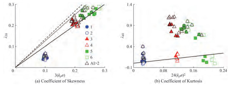Figure  5  Ensemble-averaged coefficients of skewness and kurtosis as a function of the sea state steepness k_pσ: (a) The dashed and the dotted lines represent Srokosz and Longuet-Higgins (1986) for n = 5 and n = 6. The full line stands for λ₃₀ = 3(k_pσ) (Mori and Janssen 2006); (b) The full line illustrates λ₄₀ = 24(k_pσ)² (Mori and Janssen 2006)

Download: Full-Size Img

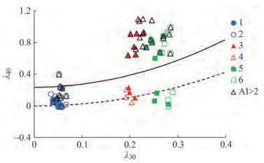Figure  6  The ensemble-averaged λ₄₀ versus λ₃₀. The dashed line is the empirical dependence of Guedes Soares et al. (2003) and the full line is the theory of Mori and Janssen (2006) for unidirectional narrowband waves

Download: Full-Size Img

Figure 5(a) shows that the second-order narrowband limit of Mori and Janssen (2006) for λ₃₀, depicted by the solid line, can provide a reasonable description for a considerable amount of cases with large vertical asymmetry from the moderate and high sea states (ε = 0.141 and 0.181), even when abnormal waves are present. However, it overestimates significantly the skewness of the lowest seas. Since the coefficient of skewness follows the physics that nonlinearity increases with the steepness in a generally linear manner, it is understandable that it approaches zero for the lowest considered steepness here, as for linear Gaussian sea with vertically symmetric wave profiles. On the other hand, with the growing energy content of the wave field, the skewness increases and reaches values of approximately 0.3 which reflects largely asymmetric wave profiles. It must be noted that oceanic measurements from storm seas typically show λ₃₀ less than 0.3, except for sea states with abnormal waves. For example, the extreme seas studied by Guedes Soares et al. (2004a) have skewness coefficients between 0.2 and 0.5, approximately. The model of Srokosz and Longuet-Higgins (1986) is presented in Figure 5(a) as a dashed line for the choice of n = 5 and as a dotted line for n = 6. As one can see, the latter choice sets an upper bound to the range of the steepest observations. The full line stands for λ₃₀ = 33(k_pσ) (Mori and Janssen 2006) and it can be observed that the skewness values are bounded by this and the line of the model of Srokosz and Longuet-Higgins (1986). Lower values of steepness are observed for the sea states measured close to the wave maker, which results from the fact that the nonlinearities build up as the wave systems travel along the tank.

Figure 5(b) presents the scatter diagram for the coefficient of kurtosis against the steepness. The widely spread data points do not show a simple dependence when third-order effects begin dominating the wave statistics. One clear result is that records with large initial wave steepness which triggered the occurrence of abnormal waves have also large positive coefficients of kurtosis. A few cases of abnormal waves associated with a coefficient of kurtosis close to zero are found in the wave fields with low initial steepness (tests 1–2). Very low estimates of λ₄₀ also characterize the steep sea states from tests 3–6 at a short distance from the wave generator (until gauge 3 which corresponds to approximately 4.8L_p). In these cases, the instability has not taken place yet which explains the observed fairly good comparison with the weakly-nonlinear model.

Figure 6 illustrates the relationship between the observed λ₃₀ and λ₄₀. The dashed line depicts the empirical fit of Guedes Soares et al. (2003) derived for records of storm seas with abnormal waves: λ₄₀ = 3.764 λ₃₀² + 0.236 and the full line represents the quadratic theoretical dependence for narrowband unidirectional waves (Mori and Janssen 2006). As one can see, the kurtosis of the largest laboratory waves is significantly higher than the predictions of the curves from (Mori and Janssen 2006), which represents a lower bound to the experimental results. However, at the lowest levels of the coefficient of kurtosis and skewness, the model of empirical dependence of Guedes Soares et al. (2003) compares reasonably well with the data.

One definite conclusion reflecting the empirical tendency in Figure 6 is that series with a large coefficient of kurtosis have also a large coefficient of skewness, as seen particularly for the cloud of sea states with abnormal waves. The dependence for the low values of λ₄₀, however, is not so straightforward, since low values of λ₄₀ are associated either with very low skewness, as for ε = 0.07, or with very large skewness, originating from ε = 0.141 and particularly from ε = 0.181. The general lack of agreement with the predictions is due to the fact that the coefficient of kurtosis, contrary to the coefficient of skewness, is largely affected by the free wave dynamics which is responsible for its significant increase.

The results in Figures 5 and 6 allow drawing the following conclusion on the dependence between the statistical cumulants and the initial wave steepness. While the largest coefficient of skewness originates from the steepest initial wave conditions, designated in the plots as tests 5–6, the largest coefficients of kurtosis belong to the moderate seas (tests 3–4). Possible explanation for this is the sensitivity of the coefficient of kurtosis to wave breaking in steep laboratory wave environments.

Next, Figure 7(a) compares the fourth-order sum Λ = λ₄₀ + 2λ₂₂ + λ₀₄ with its simplified form for unidirectional narrowband waves, Λ_app = 8/3λ₄₀, showing that generally Λ_app > Λ, although the two statistics are very close. The plot also presents the line of agreement (full line) and the actual trend (dashed line). The lowest seas follow the line of agreement, while the deviations from it increase with the steepness, as also reported by Cherneva et al. (2013) for random waves from the Marintek offshore basin.

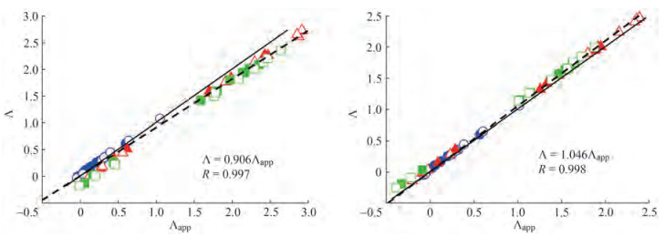Figure  7  Relationship between the ensemble-averaged Λ and Λ_app

Download: Full-Size Img

Recently, Zhang et al. (2014b) discussed the discrepancy between Λ and Λ_app for experimental and numerically simulated data, pointing out that the modulational instability alone does not play a significant role in this result if bound-wave effects are absent. This conclusion can be also validated for the current laboratory measurements by estimating the fourth-order statistics of the non-skewed free surface profiles. For this purpose, the procedure described in Fedele et al. (2010) was used to remove the vertical asymmetry due to bound-wave interactions up to third order

where $\hat{\eta}$ is the Hilbert transform of η, and β is a parameter to be determined so that $\left\langle\tilde{\eta}^3\right\rangle=0$. As a result, only symmetric corrections to the free surface are left due to free wave-wave interactions of third order which are statistically reflected by positive coefficient of kurtosis and fourth-order sum Λ.

The relationship between the estimated Λ and Λ_app for the non-skewed surface in Eq. (6) is illustrated in Figure 7(b). The comparison between Figure 7(a) and Figure 7(b) supports the conclusion that the initially observed small discrepancy in Figure 7(a) is a combined effect of free- and bound-wave nonlinearities, where the Stokes contribution has a major role. The higher-order bound-wave effects get enhanced by the nonlinear instability and eventually lead to Λ_app > Λ. This result also confirms that the cases of observed large deviations of the coefficient of kurtosis from its Gaussian value are generally results of modulational instability. Consequently, higher values of Λ are expected for an initially higher Benjamin-Feir index (see Table 1).

Figure 8 shows the ensemble averages of the coefficient of kurtosis plotted against the BFI estimates and compares the observed tendency with the quadratic dependence in Eq. (5) for narrow-banded long-crested wave fields (Janssen 2003). The theoretical formulation overestimates most of the data since it assumes nonlinear steady state at infinity while the data represent local measurements at different stages of nonlinear wave evolution. For example, some of the data points which belong to the most energetic sea states deviate largely from Eq. (5), showing sufficiently large Benjamin-Feir indices (BFI > 1) but small coefficients of kurtosis. They illustrate the wave conditions at the first three gauges (1.6–4.8L_p) where the nonlinear effects just start to develop. Figure 8 also shows as empty triangles the cases of zero-up-crossing wave maxima fulfilling the abnormality ratio of Dean (1990). One can see that only few sea states triggering abnormal waves follow the theory. Another reason for the most energetic sea states to deviate from the theory could be wave breaking affecting the kurtosis estimates.

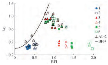Figure  8  Dependence of the coefficient of kurtosis λ₄₀ on the BFI. The empty triangles point to the cases of AI > 2

Download: Full-Size Img

Next, the variations of the coefficients of skewness and kurtosis with the distance are presented and discussed. Close to the wave generator, these statistics are nearly Gaussian which is to be expected since each free surface realization is a linear superposition of harmonics within the random amplitude/phase wave model. The significant increase with the distance of λ₄₀ and Λ is seen as a result of nonlinear instability.

Figure 9 illustrates the ensemble averages of λ₃₀ as a function of the propagated distance. The standard error, σ/N^1/2, where N = 5 is the number of data in the sample corresponding to the number of seeds for each experimental condition, is used to calculate the error bars at each gauge. It is seen that the error around the mean is quite small at all gauges, of order O(10⁻³). Moreover, the statistics do not differ significantly along the basin. The percentage variation of the overall means, (σ/µ)_λ30, can be found in Table 2. It can be seen that the smallest variation belongs to the steepest condition (tests 5–6), while the largest belongs to the lowest (tests 1–2).

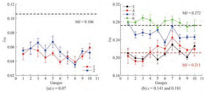Figure  9  Variation of the ensemble-averaged λ₃₀ with the distance. The dashed lines represent λ₃₀ = 3(k_pσ) (Mori and Janssen 2006) for each initial steepnessS

Download: Full-Size Img

Figure 9 also provides the estimates of the second-order narrowband model of Mori and Janssen (2006), designated as dashed lines. The theoretical predictions are shown in Table 3 together with the estimated statistical averages for each test. It can be seen that, except for tests 1 and 2, the observations are in general agreement with the theory which yields λ₃₀ = 0.211 for H_s = 0.07 m (tests 3–4) and λ₃₀ = 0.272 for H_s = 0.09 m (tests 5–6). The third-order statistics of the lowest seas, on the other hand, are quasi-Gaussian, thus they are largely overestimated by the predicted value λ₃₀ = 0.106.

The evolution along the tank of the ensemble-averaged coefficient of kurtosis is illustrated in Figure 10. It is seen that λ₄₀ is always positive when BFI is large (Figure 10(b)) while small negative kurtosis can be identified for low BFI (Figure 10(a)). The low sea states also show a slow, relatively constant increase of the kurtosis until the farthest gauge. The pattern in Figure 10(b) is different, showing a fast increase until gauge 7 (19.2L_p) followed by almost constant estimates. This trend reflects the development of third-order nonlinearity along the basin.

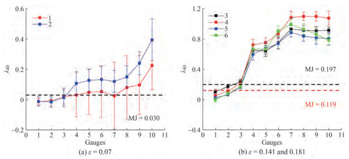Figure  10  Variation of the ensemble-averaged λ₄₀ with the distance. The dashed lines represent λ₄₀ = 24(k_pσ)² (Mori and Janssen 2006) for each initial steepness

Download: Full-Size Img

Contrary to the coefficient of skewness, the standard errors are one order higher, O(10⁻²). As can be seen in Table 2, the coefficient of kurtosis deviates largely from the mean, so that the percentage variation, (σ/µ)_λ40, exceeds 50% for the moderate and steepest seas and reaches about 100% for the lowest seas. Table 3 corroborates again that the weakly-nonlinear model fails to predict the kurtosis of the highest sea states providing λ₄₀ = 0.119 for tests 3–4 (H_s = 0.07 m) and λ₄₀ = 0.197 for tests 5–6 (H_s = 0.09 m). However, an agreement is observed for the case of H_s = 0.035 m and γ = 3 (test 1, Figure 10(a)), where the theoretical value λ₄₀ = 0.030 is consistent with the quasi-Gaussian estimate λ₄₀ = 0.056.

The pattern of change of λ₄₀ away from the wave generator agrees qualitatively with the experimental survey of Onorato et al.(2004, 2005) on the effect of modulational instability on the non-Gaussian statistics of random 2D wave trains. It also agrees with recent conclusions for 2D waves with steepness ε = 0.144 from the Marintek offshore basin (Petrova and Guedes Soares 2008). All cases of large discrepancy between laboratory data and theory have been explained with the wave unidirectionality which amplifies the contribution of higher-order effects to the wave statistics. On the other hand, the short-crested conditions suppress the wave nonlinearity, resulting in smaller λ₄₀.

4   Nonlinear wave crest and height extremes and upper bounds due to breaking

The results so far have demonstrated the importance of the coefficient of kurtosis as an indicator for increasing nonlinearity away from the wavemaker under particular wave conditions. The choice of the fourth-order statistical cumulant to mark the presence of extreme events in the wave records is supported by the spatial variation of the abnormal wave density. The abnormal wave density presented in Figure 11 is formulated as the ratio of the number of up-crossing wave heights satisfying the abnormality ratio to the total number of recorded up-crossing individual wave heights in the series. It can be seen from the plot that the number of extremely large waves in the samples along the basin is generally consistent with the spatial evolution of the coefficient of kurtosis in Figure 10. An exception to this tendency are the extremes originating from the largest initial steepness.

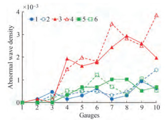Figure  11  Evolution of the ensemble-averaged abnormal wave density. Only up-crossing waves have been considered

Download: Full-Size Img

The results in Figure 11 confirm again that encountering abnormal waves is more common in moderately steep sea states (ε = 0.141). It is also interesting to observe that the least and the most energetic wave fields trigger comparable number of extreme events with the distance. The abnormal density of the moderate sea states is found to rise substantially until gauges 7–8 (approximately 19–20L_p), particularly for the peakier spectrum with γ = 6 (test 4), which clearly reflects the pattern of change of λ₄₀ (Figure 10(b)). The observed magnitude of the abnormal wave density in Figure 11 ranges between 10⁻³ and 10⁻⁴ which agrees with other laboratory findings (Onorato et al. 2006) and storm data (Guedes Soares et al. 2003). In the context of the linear wave theory, the probability of formation of extremely large waves is estimated as 3.35×10⁻⁴ which falls within the reported limits here.

In Figure 12, the ensemble-averaged abnormality ratio, AI_U, is plotted against the coefficient of kurtosis, showing a linear dependence with the coefficient of correlation R (AI_U, λ₄₀) = 0.70 which increases to R(AI_U, λ₄₀) = 0.89 if the lowest sea states are omitted. The observed correlation agrees with previous findings for abnormal waves from storm records (Tomita and Kawamura 2000; Guedes Soares et al. 2003) and laboratory measurements (Zhang et al. 2014b). The scatter shows that the extremely large waves are not only more frequently reported in moderately steep wave fields, as demonstrated by Figure 11, but they are also higher. In this particular experiment, the highest recorded extremes evolve from test 4 having ε = 0.141 and γ = 6. Contrary to field data, where the recordings show that the abnormal wave heights are concentrated over the high kurtosis range but are not particularly drawn by the highest values, here the largest waves clearly correspond to the largest λ₄₀. As for the most energetic seas over the high kurtosis range, and particularly when γ = 6 (test 6), they bring extremes around the threshold of 2 which are usually lower than or as large as the waves in the lowest seas over the low range of λ₄₀. This result finds explanation in the associated wave breaking.

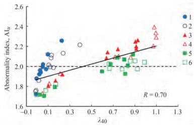Figure  12  Relationship between the ensemble-averaged coefficient of kurtosis, λ₄₀, and the abnormality index, AI_U. Both statistics are obtained as ensemble-averages over identical realizations

Download: Full-Size Img

The plot of the crest extremes versus the coefficient of kurtosis in Figure 13 shows even stronger correlation, with R(CI, λ₄₀) = 0.91, where the crest maximum normalized by the significant wave height is also known as the crest amplification index, CI = C_max/H_m0. Different threshold values can be used separately or in combination with the abnormality index to define extremely large waves, such as CI > 1.2 (Haver and Andersen 2000) or CI > 1.3 (Tomita and Kawamura 2000). Figure 13 shows that the crests exceeding these ratios are concentrated over the high kurtosis range, similarly to the largest crest-to-trough wave heights. Again, the highest measurements are result of the combination of moderate steepness and peakier spectrum with γ = 6.

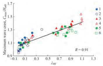Figure  13  Relationship between the coefficient of kurtosis, λ₄₀, and the normalized maximum wave crest, C_max/H_m0. Both statistics are obtained as ensemble averages over identical realizations

Download: Full-Size Img

So far, it has been discussed that the maximum observed wave crests and heights are strongly influenced by the initial wave steepness, not only because it determines the strength of the developing instabilities associated with the wave increase, but also because very steep waves can be subjected to breaking and energy dissipation. The possibility of wave breaking is discussed next by comparison of the measured wave crest and height extremes with the approximate upper limits imposed by the Miche-Stokes criteria for random wave trains.

Irregular waves with a single-peaked spectrum propagating on water of finite depth can reach maximum steepness, thus maximum wave height, as defined by Miche's limit (Miche 1944)

where k is the wave number and d is the local water depth. At infinite water depth, Eq. (7) converges to the Stokes limit for deep water regular waves.

The upper bound for the maximum wave crests, on the other hand, is obtained at a first order of approximation after substituting h_max (Eq. (7)) in the quasi-deterministic formulation of Boccotti (2000) for the expected profile of the largest observed wave:

where a is the first (global) minimum of the normalized autocorrelation function of the wave process η(t) at time $\tau^*: \rho\left(\tau^*\right) \equiv\left\langle\eta(t) \eta\left(t+\tau^*\right)\right\rangle$.

In general, the parameter a varies in the range −1 ≤ a < 0, where a → −1 represents the narrow-banded condition. As a reference, the mean JONSWAP spectrum (γ = 3.3) shows a = −0.73. The wind sea spectra are typically characterized by values of a between −0.65 and −0.73. The JONSWAP spectra at the wave generator in the present experiment demonstrates a ≈ −0.72 for γ = 3 and a = −0.79 for γ = 6.

A more conservative upper bound to the largest wave crests was proposed by Fedele and Tayfun (2009) assuming a second-order sea surface:

where μ is a normalized steepness parameter; μ = λ₃₀ /3 to O(μ²) in the most general case of second-order waves (Fedele and Tayfun 2009).

Figures 14 and 15 illustrate in semi-logarithmic scale the scatter diagrams of the σ-normalized zero-up-crossing wave height maxima h_max = H_max/σ and the normalized crest maxima, c_max = C_max/σ, respectively, versus the scaled zero-up-crossing periods, τ = T/T_m, where T_m= 2π/ω_m, ω_m = m₁/m₀ is the spectral mean frequency and m_i denotes the ith ordinary spectral moment. Each row in the figures compares results for the same sea state steepness and different peakedness parameter γ (Table 1). A total of fifty pairs (h_max, τ) and fifty pairs (c_max, τ) have been defined and used in the plots for each combination (ε, γ). They represent the wave and crest extremes at ten gauges for five identical realizations of the free surface.

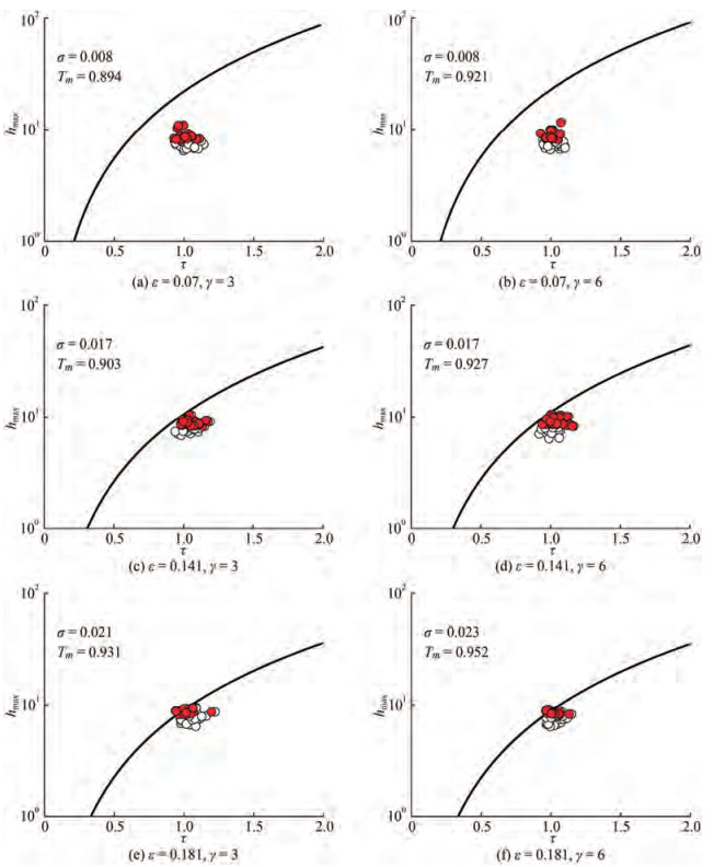Figure  14  Validation of the Miche-Stokes limit for the scatter of the up-crossing wave height maxima against the associated normalized wave periods for γ = 3 and γ = 6. The full red circles stand for the abnormal wave cases where AI_U > 2

Download: Full-Size Img

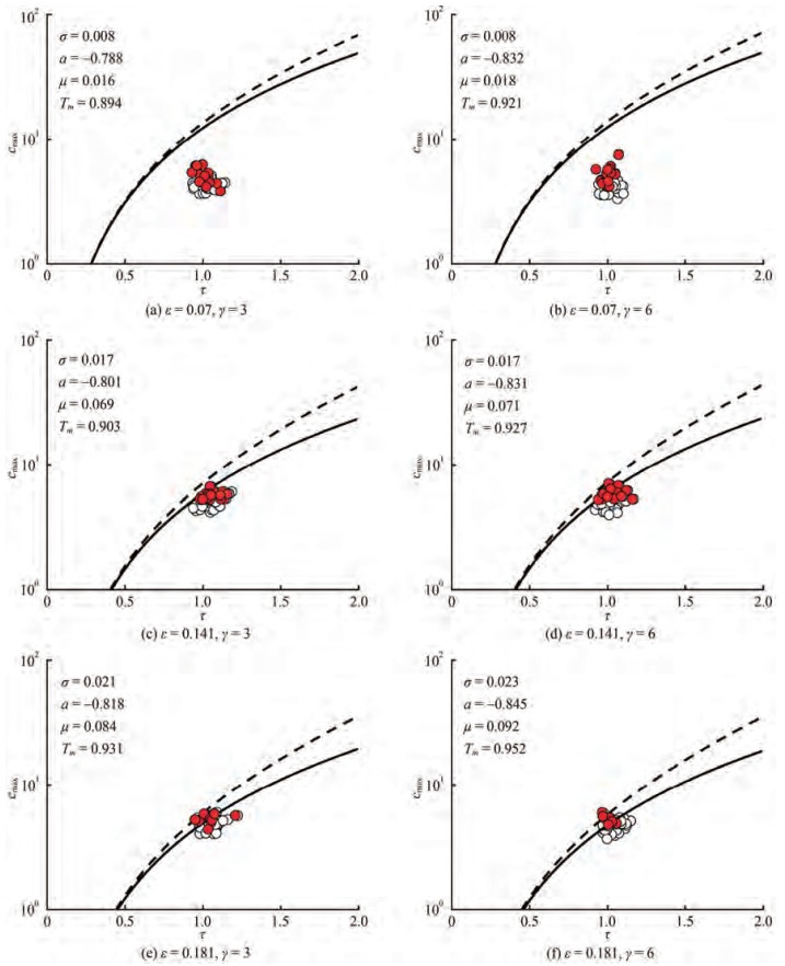Figure  15  Validation of the Miche-Stokes limits for the scatter of the wave crest maxima against the associated normalized wave periods for γ = 3 and γ = 6. The full red circles stand for abnormal waves which crest is also the largest in the sample

Download: Full-Size Img

As can be seen in Figure 14, the largest measured wave heights are between 6σ and 10σ, approximately, thus they always exceed the significant wave height (=4σ). Exceptions are tests 3 and 4 (Figures 14(c), (d)), where the lowest normalized maxima start at 7σ. The full red circles in the plots outline the abnormal wave cases as they exceed the threshold AI_U = 2. The full lines define the upper bounds predicted by Eq. (7) where the scaling parameters T_m and σ (provided in the plots) represent statistical averages for every steepness case ε. Abnormal waves exceeding the upper boundary can be observed only in the most energetic and steep wave environments (Figures 14(e) and (f)). This explains the reduced number of large-amplitude events registered in these particular sea states which is comparable with the abnormal wave density for ε = 0.07, as illustrated in Figure 11. Moreover, it is not only the number of very large waves that repeats the spatial evolution of λ₄₀ but also their magnitude. Thus, these waves are eventually as high as the waves originated from ε = 0.07.

Figure 15 compares the sampled crest maxima and the associated crest periods against the approximate bounds c_max1 (Eq. (8)) and c_max2 (Eq. (9)). In this case, the full red circles represent particular cases of abnormal waves which crest is also the largest in the time series. This situation is reported for 74% of the abnormal wave heights. Figure 15 shows similar tendency for the largest crests, as for the largest wave heights. The lowest sea states (Figures 15(a), (b)) bring crest maxima ranging between 3σ and 7σ which stay largely underestimated by the upper limits. On the other hand, the crest extremes in sea states with ε = 0.141 and ε = 0.181 (Figures 15(c)–(f)) begin from 4σ up to approximately 7σ and the crests of the abnormal waves do exceed the limits, including the more conservative approximation, especially for the steepest conditions in Figures 15(e) and (f).

The comparisons in Figures 14 and 15 confirm the relative validity of the Miche-Stokes criteria as an upper bound for the shape of the largest waves in a random wave field, similarly to results from previously analysed laboratory measurements (Cherneva et al. 2009, for single wave systems; Petrova and Guedes Soares 2014, for crossing seas) and field data (Tayfun 2008). However, it is always noted that these criteria cannot serve as a consistent indicator for incipient wave breaking.

5   Conclusions

The performed study show that the generated wave fields become increasingly nonlinear, sometimes exceeding significantly the predictions of the Gaussian and second-order models and empirical dependencies, conditional on the Benjamin-Feir index of the input JONSWAP spectra.

One typically reported result associated with four-wave quasi-resonant interactions between free wave modes has been observed: the spectral evolution over the distance. Comparisons at certain locations, corresponding to different stages of the developing instability, allow detecting the broadening of the studied spectra around the peaks and the peak downshift for moderate and high initial steepness in combination with peakier spectra. It has been observed that the downshift of the peak along with the observed reduction of the high-frequency tail in steeper seas can be a combined effect of nonlinear instability and energy dissipation due to wave breaking. The relevant Miche-Stokes limits showed that the extreme wave heights are always higher than the significant wave height but do not in general exceed the theoretical thresholds, except for the abnormal wave cases with abnormality index AI_U > 2, triggered by the combination of ε = 0.141 and γ = 6 (test 4). The largest crests, however, are more sensitive to nonlinearity and breaking, and the scatter diagrams confirm this, showing that the sampled maxima are frequently over the approximate limits.

One significant effect of quasi-resonant modulations on the wave statistics is the monotonically increasing coefficient of kurtosis away from the wave generator when BFI is large. Moreover, the largest waves are found to follow this pattern, thus they are more frequently encountered at larger distances, after approximately 14.4L_p (gauge 4), as revealed by the abnormal density parameter. This parameter also validates results from previous laboratory experiments that the largest number of abnormal wave cases are triggered by sea states of initially moderate steepness.

It has been also found that the largest wave heights and crests of waves classified as abnormal, either because AI_U > 2 or the crest amplification index exceeds a prescribed value, are drawn by the largest kurtosis which somewhat contradicts previous conclusions on field data where the abnormal waves were spread over a range of large kurtosis values (Petrova et al. 2006).

An interesting result is that the nonlinear behaviour of the most energetic and steep seas is very similar to that of the lowest seas. It can be explained with loss of energy due to breaking which reduces the magnitude of the expected extremes and thus have critical effect on the coefficient of kurtosis, as reflected by the slightly smaller estimates over the last four gauges (Figure 10) for ε = 0.181 and γ = 6 (test 6).