1   Introduction

Accurate prediction of roll damping and roll motion is essential for operational and safety considerations and is a primary naval architecture concerns. The roll motion is a nonlinear phenomenon in which the vortices intensity depends on the amplitude of the roll motion. As a result, linear method's accuracy decreases, especially near and at the resonance area, where the marine vehicle might exhibit largeamplitude roll motions that may endanger crew safety, cargo on deck, and the vessel itself, and even might lead to the ship capsize at worst cases. Therefore, the prediction and study of the roll motion are significant. However, the roll motion predictions accuracy lags behind that of heave and pitch motions. That is due to the importance of viscous effects in this motion mode, especially near the resonance. Besides, in the second generation intact stability criteria (SGISC) at the International Maritime Organization (IMO), an accurate roll damping estimation is essential to assess ships' vulnerability to several dynamic instabilities.

The roll damping is related to the flow around the hull and is hard to be calculated theoretically. In most cases, the roll motion is studied using potential flow methods by adding an artificial viscous damping term to account for the viscous effects. Model tests or semi-empirical formulas could estimate the viscous damping term.

The main experimental tests to evaluate the roll damping are roll decay, forced roll and excited roll tests. A roll decay test is, however, the most common one. More advanced techniques, such as forced roll and excited roll tests, are also used and reported recently. However, they require more equipment and mechanical systems for forcing the roll motions. Therefore, roll decay is still the most available test to estimate the roll damping. Although the roll decay can be performed quit easily, it still needs a scaled ship model, a test basin and motion recording sensors. In the semi-empirical formula by Ikeda, the roll damping is divided to wave damping, lift damping, friction damping, eddy making damping and bilge keel damping. Potential flow theory could calculate only the wave damping, and other parts should be obtained from other methods. Semi-empirical methods like the Ikeda method is still widely used in the estimation of the roll damping. But it is inaccurate in many cases, like the geometries with a shallow draft. Such limitations urge the researchers to use the fully nonlinear RANS-based methods to calculate the roll damping terms. CFD codes and tools can be used as an alternative to the physical model tests.

Recent progress in CFD code development and its application in naval architecture will likely revolutionize many sections in this discipline. Naval architecture sub-disciplines for resistance and propulsion, maneuvering and seakeeping, and ship design process could be addressed directly by CFD solvers with high precision. The only drawback for such methods is still the expensive computations with long computational time, making the calculations impractical in some cases. One solution to this is the combination of CFD methods with fast potential-based methods. Potential based numerical simulations using CFD code contributions have both low cost and high accuracy in the calculations. These methods have become a hot subject in seakeeping research activities, recently.

Application of CFD methods in resistance and propulsion is the most advanced one with more than three decades of experience. It has shown a reasonable accuracy, as shown in different studies in the literature. CFD methods have been used for optimization purposes for different objective functions in the ship design stages as well. The application of CFD methods in the maneuvering and seakeeping is less mature due to the complexities of unsteady flow, ship motions, highly nonlinear environment (steep incident waves, wave breaking, green water, etc.) and also expensive computations. Some steady maneuvers have been studied with CFD methods extensively, but more unsteady maneuvers are rare. Typical seakeeping analyses are based on the assumption of small amplitude motions based on potential flow theory. 6-DOF motion is, in general, reduced in two sets of equation and is solved in the frequency domain. The viscous roll damping is also incorporated in the equation using empirical methods or experimental data. Such methods are limited to a range of geometry, frequency and also parameters from empirical techniques or experimental data. Simulations in the time domain can be used for larger roll motions, but still is dependent on the empirical methods (which are not accurate in many cases) and experimental data (which might not always be available). Therefore, the need for a valid and reliable method for predicting the viscous roll damping is felt. The development of time domain potential-based solvers combined with CFD codes (for calculating the viscous roll damping) could be an excellent solution to this gap. It is obvious that the 6-DOF simulation using CFD codes, is not practical in terms of computational time and resources. But the highest advantage from CFD code, could be taken in terms of viscous roll damping. The study of roll motion using CFD, is not only a solid step forward in seakeeping analysis, but also an efficient and accurate one (comparing to semi-empirical methods and model tests). Due to the developments in terms of computational resources available, the simulation based on CFD is now possible but is still very limited.

Chen et al. (2001) performed a Reynolds-Averaged Navier-Stokes numerical method in conjunction with a chimera-domain decomposition approach for time-domain simulation of large amplitude ship roll motions. They investigated a six degree of freedom motion for time domain simulation of free roll decay for a ship and a free-floating pontoon. The simulation was evaluated in 6 different loading conditions i.e. two drafts (1.22m, 1.83m) and three center of gravity (2.78m, 3.11m, 3.4m) and free decay roll simulations were performed for all six test cases and compared with the available experimental data. However, they did not discuss the details of computational domain, mesh and verification and validation of the results.

Wilson et al. (2006) performed an unsteady RANS simulation for computing the roll decay motion and flow field for a surface combatant with and without appendages using CFD SHIP IOWA. Roll decay simulations are performed for three cases: the bare hull (i.e., without rudder, shafts, propellers, etc.) at medium speed (Fn=0.28, Re = 4.65e6) at low speed (Fn=0.138, Re = 2.56e6) and bare hull geometry appended with bilge keel at low speed. They investigated verification and validation based on the procedures presented by Stern et al. (2001).

Yang et al. (2012) investigated numerical simulations of DTMB 5512 without appendages free roll decay in calm water and the initial roll angle 10.0° at two Froude numbers (Fn = 0.138, Fn = 0.28) using commercial software Fluent and RANS solver with a dynamic mesh technique. The authors concluded that for free decay, the natural periods of ship model advancing at different speeds are calculated with an error of 1.3%‒2.5%. However, they did not discuss the details of the computational domain and mesh.

Avalos et al. (2014) investigated the roll damping decay test for a middle section of Floating Production Storage and Offloading (FPSO) with bilge keel by the numerical solution of the incompressible two-dimensional Navier—Stokes equations, and the governing equations solved using the finite volume method and the upwind Total Variation Diminishing (TVD) scheme of Roe—Sweby. The simulations were focused on the bilge keel shape and types. They concluded that the agreement between numerical and experimental results for the decay test was much better for the case with bilge keel than without and the numerical results shown the increase of damping coefficient with the height of the bilge keel.

Zhu et al. (2015) investigated a 3D simulations of free decay roll motions in calm water for the ship model DTMB 5512 without appendages by Reynold averaged Navier-Stokes (RANS) method based on the dynamic mesh technique at three different Froude numbers (0.138, 0.28, 0.35) using Fluent software. They also estimated the numerical errors and uncertainties. The authors showed that level of numerical uncertainties 1.818% and 1.532%, and comparison errors of 1.21% and 1.43%, respectively, also error in natural period showed a error between 1.3% and 2.5%.

Mancini et al. (2018) simulated the free roll decay tests for the bare hull naval ship DTMB 5415 at zero speed with different initial heeling angle of 4.0°, 13.5°, 19.58° and 24.5° using a RANS solver. They did the verification and validation for grid, and time step according to the CGI approach.

Jiao et al. (2021) investigated ship motion behavior in bi-directional cross waves by a computational fluid dynamics (CFD) solver. The characteristics of cross waves are analyzed theoretically and by CFD verification at first. Then ship nonlinear motion responses and green water on deck induced by cross waves are systematically analyzed on a S175 containership model in different wave scenarios. Some useful insight and guidance for the safety operation of ship when encountering cross seas are also provided. Jiao and Huang (2020) investigated the slamming loads in bi-directional cross waves in addition to the ship motions for the same containership model. Huang et al. (2021) compared the seakeeping behavior for the same S175 containership model in multi-directional waves against uni-directional wave. Their comparative results indicated that ship motion response in bi-directional waves is generally larger than that in uni-directional waves. Moreover, severe bow slamming and green water under bi-directional waves were also observed and investigated.

Sadeghi and Hajivand (2020) investigated the effect of a canted rudder system on the roll damping of a twin-screw naval vessel. They used a RANS solver for the roll damping investigation and performed several roll decay simulations in different situations to get the damping in different scenarios. They concluded that the roll damping increases for higher forward speed as the angle of the canted rudder system increases. One of the effective parameters on the roll motion amplitude of the ship is metacentric height. Hasanvand et al. (2019, 2021) Have studied the time history of the roll motion in ship maneuver and its dependence on the metacentric height by simulating 6-DOF ship turning and zigzag maneuvers for different rudder profiles for a container-ship model. It is observed that with increasing metacentric height, the amount of roll decreases severely.

Ghamari et al. (2015) investigated the parametric roll phenomena for a container vessel using a nonlinear solver. They used the Ikeda empirical method to estimate the roll damping and the results they got showed a good agreement with the experimental results in terms of parametric roll occurrence and the roll amplitude. Ghamari et al. (2017); Ghamari (2019); Ghamari et al. (2020) investigated the nonlinear roll motion in the parametric resonance area for different scenarios for a fishing vessel. They conducted many experiments and simulations in their analysis. They extract the roll damping from the experimental roll decay tests and used them in the numerical simulations. They checked the extracted damping by reproducing the experimental roll decays numerically and comparing the results with the experimental data. They also captured most of the cases with parametric roll occurrences in their analysis. Ghamari et al. (2021) also investigated the roll moment due to a free-surface anti-roll tank experimentally and numerically. This tank could be used as extra damping device in roll motion.

In this study, the free decay roll motion is studied using CFD simulations. The novelty of this paper is using CFD precision in extracting the roll damping and using the fast calculations of the potential-based solvers at the same time. It is obvious that due to the limited computational resources and also the long and time-consuming computations in CFD-based solvers, the seakeeping simulations are not that practical. But using the suggested hybrid method could be a fast and precise solution to many seakeeping analyses for different vessels. In this paper, the obtained results for a fishing vessel are validated against the experimental data. Afterwards, the obtained roll damping is used in the time domain simulation of the fishing vessel in the incident waves and validated against the experiments. The present study focuses on the nonlinear time domain simulation for the ship motions using the CFD-derived viscous roll damping. The simulations are performed for a fishing vessel in the parametric resonance area and the results are validated against the experimental results. In the section 2, the model and the experimental setup is explained. Section 3 describes the CFD simulation setup which is followed by verification and validation of the solver. Section 4 shows the obtained results for the CFD parts. Extracting the damping from the CFD results and using them in the hybrid method for free decay cases and cases in waves are presented in section 5. Finally the main results are summarized and the conclusions are drawn.

2   Model and experimental setup

A comprehensive experimental investigation on the parametric rolling of a fishing vessel was carried out at the CNR-INSEAN basin No. 2. In this experimental campaign, different roll decay tests were performed as well. The dimensions of this basin are: length × width × depth= 220 m × 9 m × 3.6 m. The wave basin is equipped with a flap wave-maker, hinged at a height of 1.8 m from the bottom. The experiments performed on a scaled model (1:10) of a Norwegian fishing vessel. The model hull was made out of wood and was used for different types of experiments which will be explained in this chapter. The vessel model (INSEAN model C2575) is built at CNR-INSEAN in scale 1: 10 and reproduces a medium sized Norwegian fishing vessel (SFH112). The body plan with skeg and a 3D view of the C2575 model are shown in Figures 1 and 2, while Table 1 reports the detailed geometric and hydrostatic properties. The bilge-keel effects are not examined in this paper because they would require a dedicated study in combination with the other parameters examined in the present paper. This is left for a future in-depth study. However the effect of the bilge keel on the roll damping in the same ship model has been investigated experimentally and numerically in Aarsaether et al. (2015).

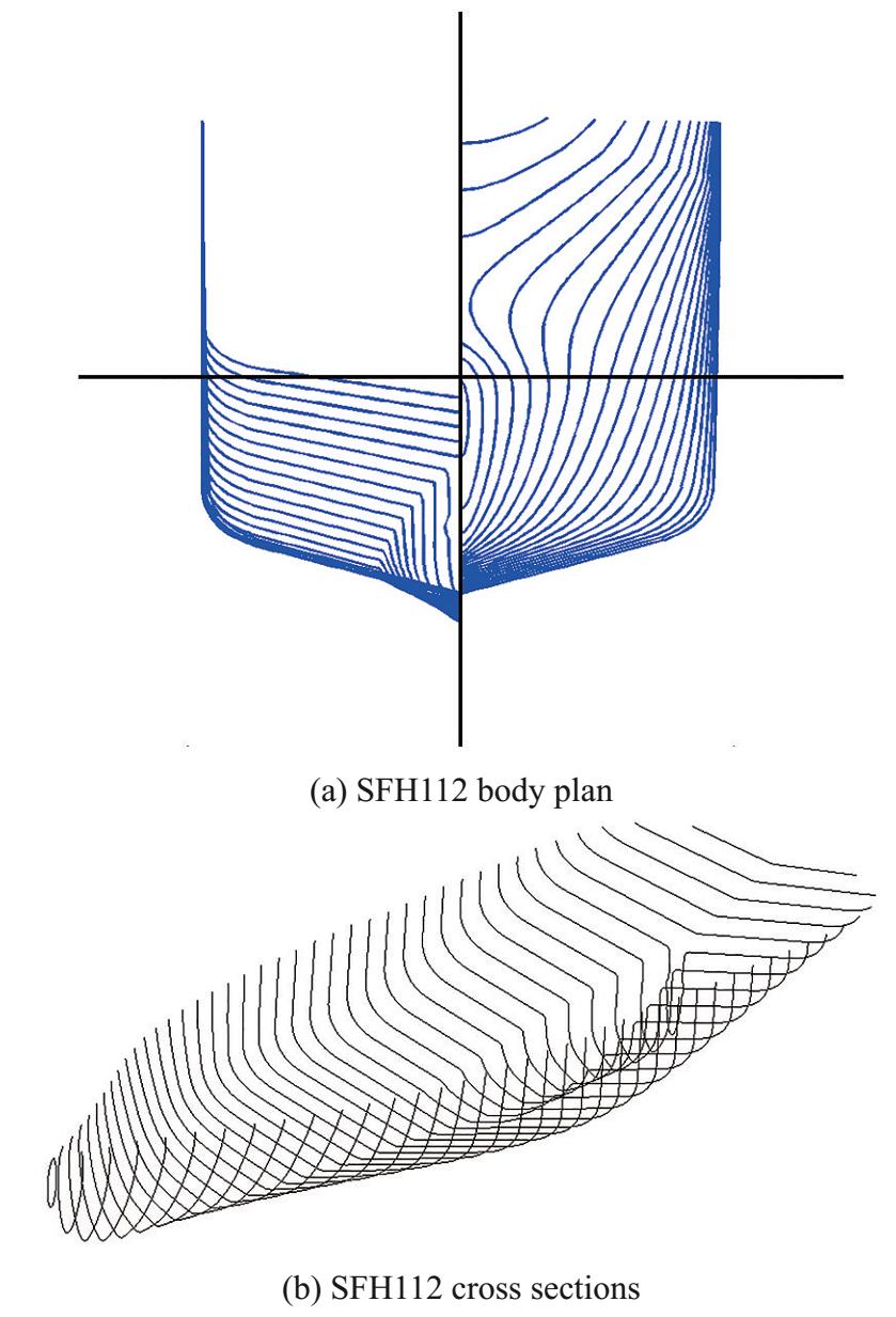Figure  1  SFH112 fishing vessel body plan and cross sections

Download: Full-Size Img

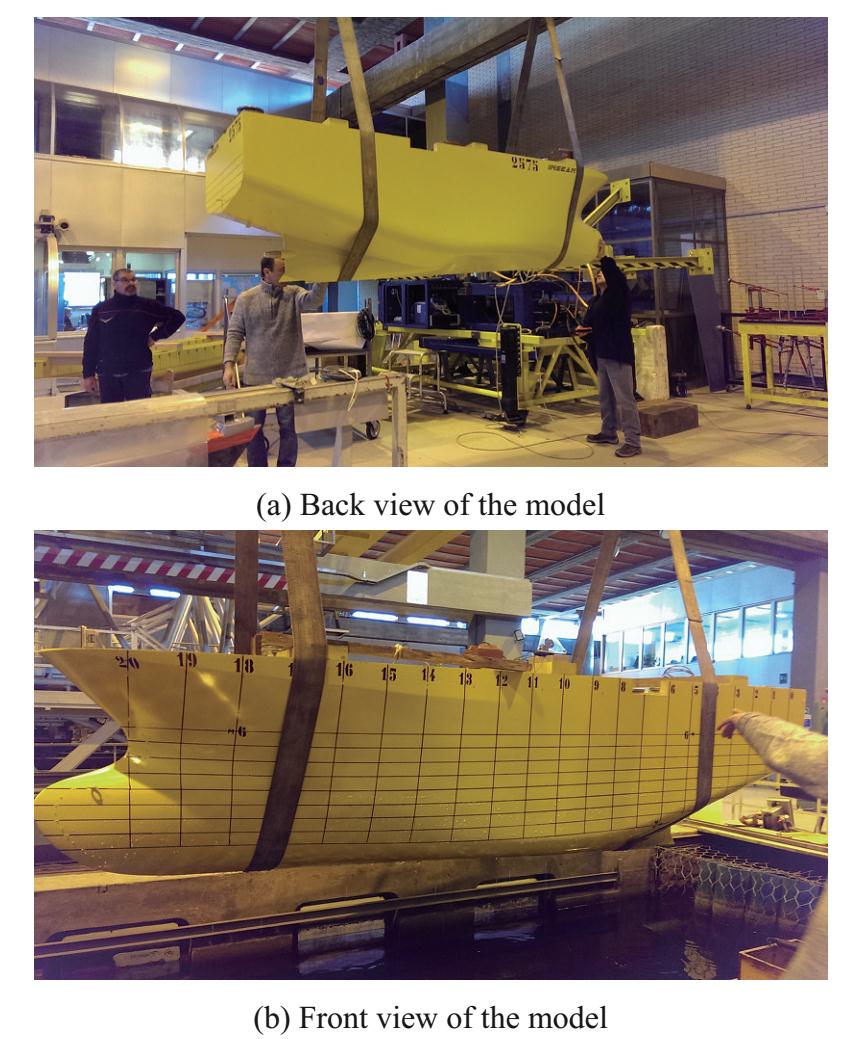Figure  2  Pictures of the SFH112 model at CNR-INSEAN basin

Download: Full-Size Img

Fishing vessels in Norway tend to become wider in order to increase the payload due to regulatory length limitations, so SFH112 vessel is also fairly wide. The midship region of the vessel lacks the uniform sections seen on larger vessels and the body plan shows a vessel where the region of similarly shaped sections is short. This makes the vessel more vulnerable to parametric roll due to larger variation of the water-plane area in waves with wavelengths in the order of the ship length. The main characteristics of the model are shown in Table 1.

3   CFD simulation setup

3.1   Fluid flow modeling

Unsteady, viscous, turbulent, and incompressible flow around a rolling ship is governed by continuity and Navier-Stokes (NS) equations. The SST k-ω turbulence model that provides a good compromise among accuracy and computational cost has been used to consider more precisely the effects of flow turbulence, especially the formed eddies near the hull. Moreover, the free surface between water and air was captured through multiphase VOF method via solving an additional transport equation for an extra scalar variable known as the volume fraction. An HRIC scheme is correspondingly has been used to track sharp interfaces between two immiscible fluid components.

3.2   Numerical details

Due to the unique advantages of the finite volume method in solving computational fluid dynamics problems, this method has been used to discretize the governing equations. The dimensions of the computational domain in which the discretize equations are solved are determined according to the ITTC Recommended Procedures and Guidelines (2014) in such a way as to avoid undesirable effects such as reverse flow at outlet, blockage effect at wall sides, and shallow water effects at bottom boundary. Within the computational domain, an internal region, known as overset, around the ship is defined to consider the roll motion. The transmission of fluid flow data between overset region and the computational domain at each time step is based on the overset technique. Overset technique required two different regions i.e. background and overset. A general view of the Background and Overset is displayed in Figure 3. Also, the dimensions according to Figure 3 are compared with the previous researches in Table 2. Assigning proper boundary conditions for the main computational domain, body, and overset area has a large effect on the results. Table 3 and Figure 4 indicate the type of boundary conditions.

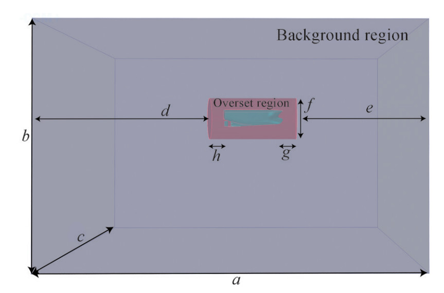Figure  3  Displaying background and overset dimensions.

Download: Full-Size Img

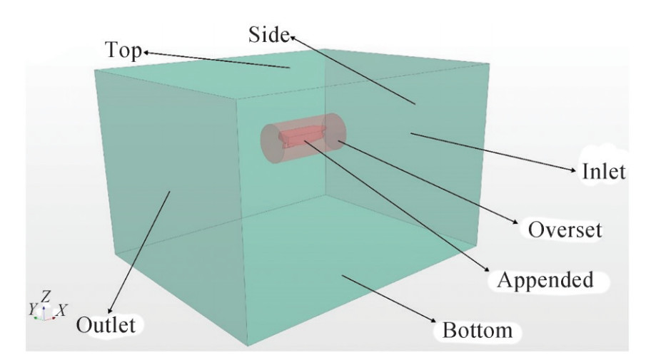Figure  4  Boundaries of the computational domain

Download: Full-Size Img

Simulations are performed using a numerically and computationally efficient and robust unstructured meshing technique, by ability to correct local improvement (near the hull and at free surface). A very slow expansion rate has been used to maintain mesh connectivity. An overall view of the mesh in computational domain and around the body hull is shown in Figures 5 and 6.

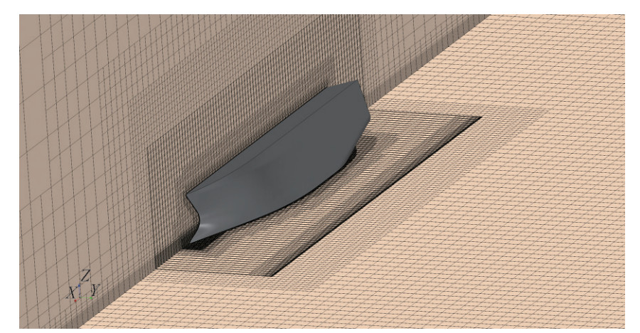Figure  5  View1 of the mesh around the hull

Download: Full-Size Img

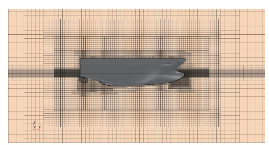Figure  6  View2 of the mesh around the hull

Download: Full-Size Img

As an important part of roll motion attenuation due to viscosity damping, a prismatic boundary layer technique has been used for the boundary layer region around the hull. Twenty prismatic layers with 1.2 expansion ratio are used to discretize this area. For fine grids near the walls in the viscous sub-layer RANS equations are resolved (y⁺ < 1) and the wall functions are used for the coarser grids (y⁺ > 30). The distribution of y⁺ for the fine mesh on the hull is displayed in Figure 7.

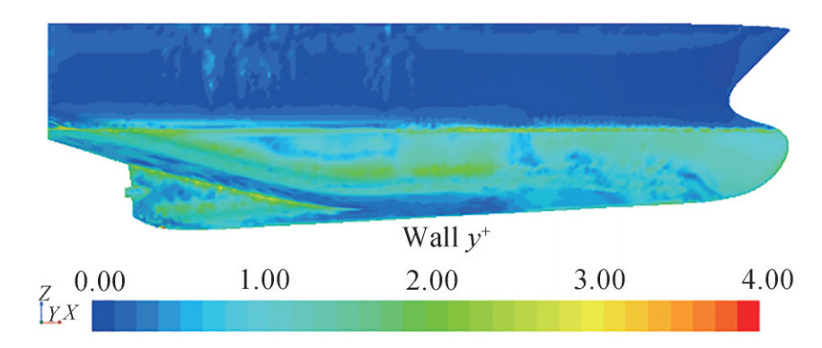Figure  7  Wall y⁺ distribution on the hull

Download: Full-Size Img

The DFBI module is used to solve the 1-DOF dynamic equation of roll motion in the free roll decay simulation. Velocity and pressure as unknown quantities are correspondingly calculated using an unsteady implicit solver. An algebraic multi-grid (AMG) algorithm is applied to accelerate the convergence of the solution.

3.3   Verification and validation

3.3.1   Verification

Numerical simulation can contain some errors that cause the numerical simulation results to differ from the actual values. Correspondingly, it is essential to evaluate the precision of the outputs by performing proper verification and validation analyses. Simulation error (E) and uncertainty (U) in a numerical solution can be caused by numerical or modeling sources. E and U can be expressed as follows Stern et al. (2001):

where S and T are exact and numerical solution, respectively. δ_SM and δ_SN also expresses modeling and numerical errors, respectively. And correspondingly uncertainty is de fined as follows: the simulation numerical error and uncertainty were decomposed into contributions from iteration number, grid size, time step, and other parameters.

where U_S is simulation uncertainty and U_SM, and U_SN are modeling and numerical uncertainty, respectively. Simulation numerical divided into contributions from grid size (U_G), time-step (U_T), inner iteration (U_I), and other parameters. The verification procedure proposed by the ITTC has been used through convergence studies. Previous research in free roll decay simulations has shown that the dependence of the results on inner iteration changes compared to grid and time-step is negligible (Wilson et al. 2006). Accordingly, in all simulations, the number of inner iterations was set to 10.

Grid and time-step convergence studies are performed by means of multiple solutions which are refined systematically with a reasonable refinement ratio $ r = \sqrt 2 $ (ITTC Recommended Procedures and Guidelines 2017). Three modes of convergence can occur: Monotonic convergence (0 < R < 1), Oscillatory convergence (R < 0) and divergence (R > 1), where R is convergence ratio. Normally, the preferred state is monotonic convergence, in which case errors and uncertainties can be estimated via generalized Richardson extrapolation approach.

For grid convergence study three grids has been generated and verification is performed. The twelfth roll peak has been selected for comparison. The base size, total grid numbers for overset and main computational domains, and computed fifth roll peak are given in Table 4. Using Table 5, the value of the convergence ratio is calculated to be 0.57, which indicates the monotonic convergence. As a result, Richardson's method can be used. In Table 5 the values of the order of accuracy (P) and grid convergence index (GCI) are presented, these values are calculated based on the definitions provided in the ITTC Recommended Proce dures and Guidelines (2017). The theoretical value for P is 2 and the variance in the obtained value is due to turbulence closure modeling, model nonlinearities, as well as grid quality. Furthermore, roll decay time history for different grid cases are illustrated in Figure 8. It can be seen that the results of these simulations, which have been performed with a medium time step (0.002 s), are very close to each other, especially the results of medium and fine mesh. As well, three grid meshes around hull for initial angle 10.81° are compared in Figure 9 to Figure 11.

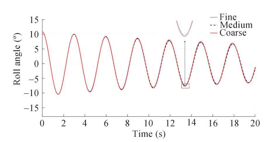Figure  8  Free roll decay for three different grids with an initial angle 10.81° at Fn = 0

Download: Full-Size Img

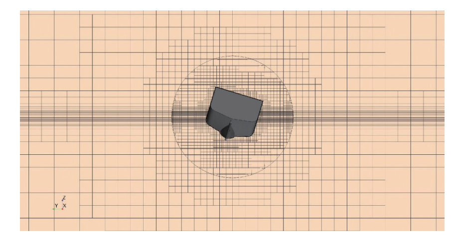Figure  9  Coarse mesh on the model

Download: Full-Size Img

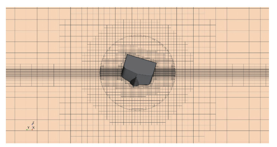Figure  10  Medium mesh on the model

Download: Full-Size Img

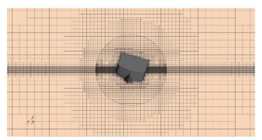Figure  11  Fine mesh on the model

Download: Full-Size Img

In a similar way, the verification process for time-step can be done. The importance of this issue increases because the simulation of roll decay motion has a high sensitivity to time step. Time step study is evaluated through roll peak solutions on three systematically refined time steps. These three simulations are performed for medium grid and fifth roll peak for three cases are presented in Table 6. After calculating the value of the convergence ratio and ensuring the achievement of monotonic convergence, the order of accuracy (P) and grid convergence index (GCI) were calculated and are given in Table 7. Furthermore, roll decay time history for different time steps are compared in Figure 12.

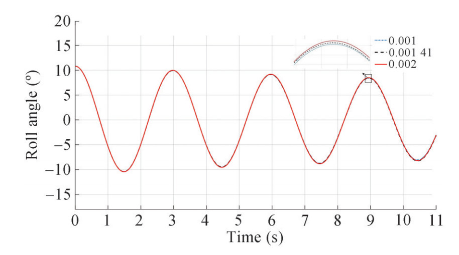Figure  12  Free roll decay for three different time step with an initial angle 10.81º at Fn = 0

Download: Full-Size Img

Although the results show that the difference between the outputs of fine and medium spatial and temporal discretization is negligible, the computational time to achieve the fine solution is much longer. Accordingly, in order to balance the accuracy and cost in the final simulations, the medium grid and medium time-step has been used which are consistent with the ITTC Recommended Procedures and Guidelines (2014) for periodic tests simulation.

3.3.2   Validation

Numerical solution results should also be compared with experimental data for validation. Hence, experimental results provided by Ghamari (2019) for 1-DOF bare hull condition are used for validation. Numerical and experimental time histories of roll decay at 10.81° are compared in Table 8. As it can be seen from Table 8, the overall agreement is perfect in both roll frequency and amplitude. The biggest difference between the peak time is less than 0.2% and in the roll amplitude in the peaks is less than 1.42% that shows a good agreement among CFD and EFD results.

4   Simulation results

In the following, the results obtained from the roll decay test simulation using two numerical methods based on viscous and inviscid flow solvers are presented. Given that the free roll decay test results are for zero forward speed, the main focus of the simulations is on this case. However, simulations have also been performed to examine the effect of the degree of freedom and forward speed. Also, the effect of two well-known turbulence models of k-ε and k-ω SST on the damping of roll motion has been investigated by simulating the free roll test for the initial angle of 10.81° at Fn=0, the comparison of which is given in Figure 13. It can be seen that the numerical results are within 1% difference. Due to good trade-off between computational cost and precision, all simulations were conducted with the RANS k-ω SST turbulence model in combination with wall functions for the turbulent boundary layer. The comparison of the results using the two turbulence models are shown in Figure 13.

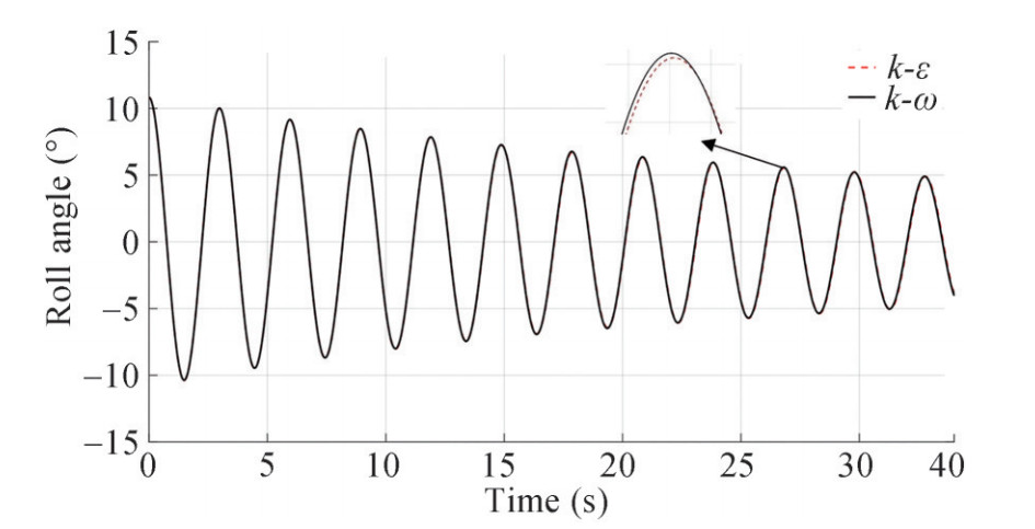Figure  13  Free roll decay using k-ε and k-ω turbulence models with an initial angle 10.81° at Fn = 0

Download: Full-Size Img

The obtained results by RANS for 1-DOF test cases with the initial roll angle 10.81° and 16.76° are shown in Figures 14 and 15, respectively. Comparison of results with EFD data is also provided. The cases are performed for the hull with zero forward speed. As it can be seen from these figures, the overall agreement is perfect in both roll frequency and amplitude. As stated in the validation section, the biggest difference between the peak times is less than 0.2% and in the roll amplitude in the peaks is less than 2.7%.

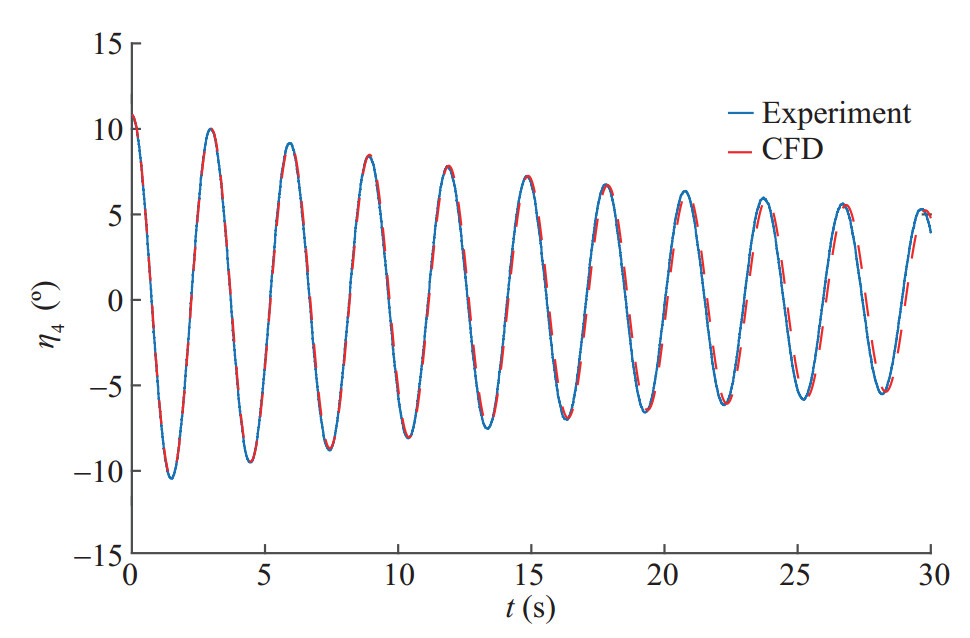Figure  14  Comparison of roll decay of experimental results and CFD results for case C529

Download: Full-Size Img

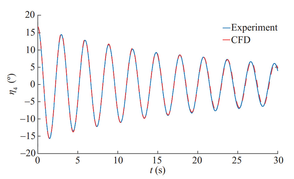Figure  15  Comparison of roll decay of experimental results and CFD results for case C541

Download: Full-Size Img

And the comparison of results for case C541 is shown in Figure 15.

Roll decay time history obtained at inclination angle 10.81° for different ship forward speed is presented in Figure 16. It is clear from the comparison of these results that with increasing forward speed the damping rate of the roll motion increases significantly. An increase in the forward speed leads to a change in the pressure distribution over the bilge region and followed by an increase in the hull lift component. On the other hand, forward speed increases the rolling period of the vessel. Hydrodynamic roll moment produced by the hull is presented in Figure 17 for different forward speed.

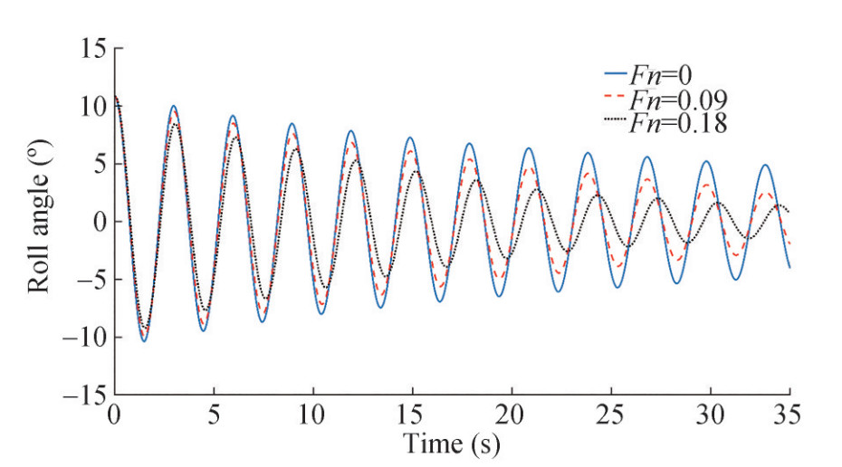Figure  16  Comparison of CFD results for roll decay at different forward speed

Download: Full-Size Img

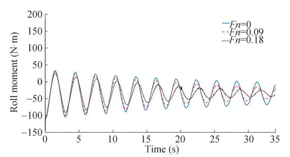Figure  17  Comparison of CFD results for hydrodynamic roll moment at different forward speed

Download: Full-Size Img

To consider the effect of other degree of freedom for the initial angle of 10.81° and at Fn=0, the roll decay test is also simulated as 6-DOF. The roll decay time history diagrams for 1-DOF and 6-DOF are compared in Figure 18 that is found the differences in roll amplitudes are insignificant. The effect of DOF has been investigated by Irkal et al. (2016) and Mancini et al. (2018) and it can be concluded that this effect depends on hull geometry and metacentric height. The diagrams of the motions of the heave, pitch, sway, surge and yaw are also shown in Figures 19 and 20. It can be seen that after 5 s of physical time, sway, yaw and surge start to deviate. However, the heave and pitch motions are insignificant compare to the other motions.

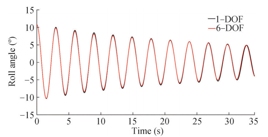Figure  18  Comparison of the roll decay with1 and 6-DOF system for case C529

Download: Full-Size Img

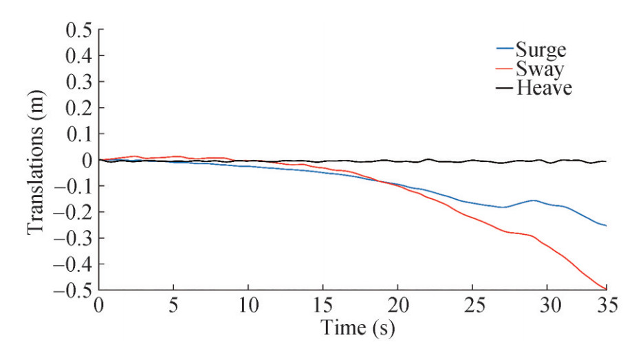Figure  19  Motions (Surge-Sway-Heave) time histories of the roll decay case with for case C529

Download: Full-Size Img

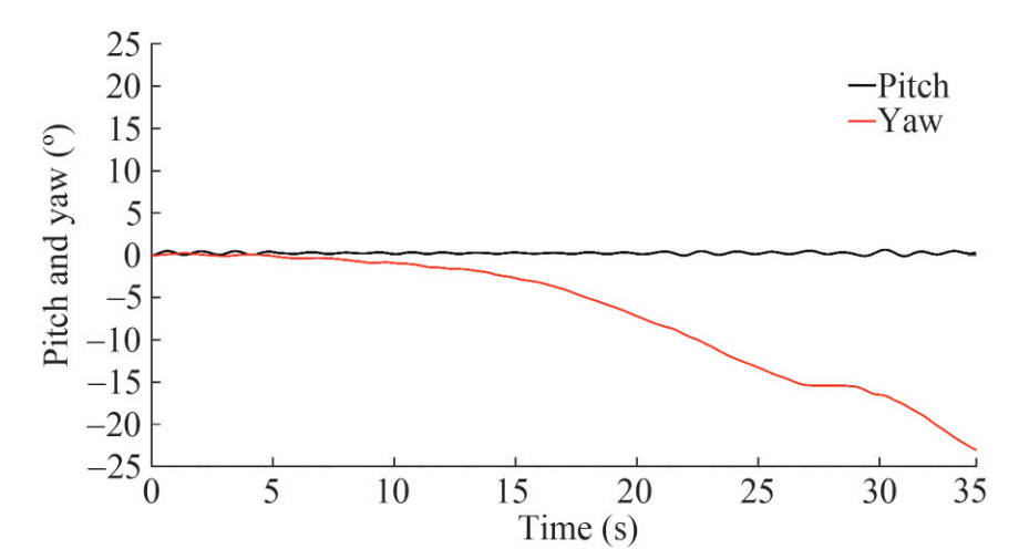Figure  20  Motions (Pitch-Yaw) time histories of the roll decay case with for case C529

Download: Full-Size Img

Figures 21 and 22 show the time history of the roll angle and hydrodynamic roll moment produced by the hull at Fn=0 for viscous and inviscid solvers. It can be seen that the damping rate of the ship roll in the viscous solver is a bit higher because the ship roll moment is higher in viscous flow conditions. Also, comparing these figures demonstrates that the hydrodynamic roll moment generated by the hull is almost 180° out of phase with the roll motion. Therefore, hull moment has its most effects in the added inertia and negligible damping effect.

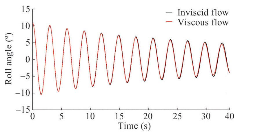Figure  21  Roll decay comparison with viscous and inviscid solvers for case C529

Download: Full-Size Img

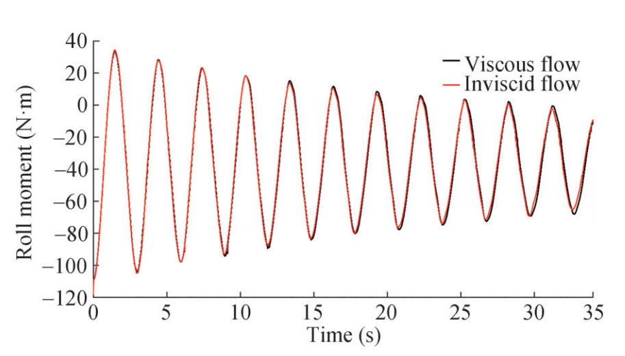Figure  22  Hydrodynamic roll moment in free roll decay test with viscous and inviscid solvers for case C529

Download: Full-Size Img

5   Results of the hybrid solver

5.1   Results in free decay

In this section we try to use the results obtained by CFD simulations and use them in the fast potential solver. In this way we can use the precision of the CFD in terms of estimating the roll viscous damping correctly, and the fast simulations of the potential-based solver at the same time. First we get the viscous damping from the CFD results and then we use them in reconstructing the same roll decays. Afterwards, we try to use the obtained damping in an important seakeeping problem (parametric rolling study) and try to analyze the parametric rolling occurrence for the vessel in head sea waves at Fn=0. The obtained results for the parametric rolling part is validated against experimental results provided by Ghamari (2019).

The comparison of the results for the two cases at Fn=0 against the experimental data showed a good agreement, now we can try to extract the roll damping to use in the next studies for this vessel. It is a common engineering practice to extract the damping coefficients from the free decay tests. In this regard, the damping is assumed to be constant with respect to the amplitude of oscillation and the motions is normally considered as uncoupled 1-DOF equation as follows, Faltinsen (1993):

where X_n is the nth oscillation and there is one half period T_m/2 between X_n and X_n+1. By plotting the $ \frac{2}{{{T_m}}}\log \left({\frac{{{X_{n - 1}}}}{{{X_{n + 1}}}}} \right)$ term against $ \frac{{16}}{3}\frac{{{X_n}}}{{{T_m}}}$ term for different n and fitting a straight line, the linear and qudratic damping could be extracted. The points extracted from both decay tests in Fn = 0 is plotted and the fitted line is drawn in Figure 23.

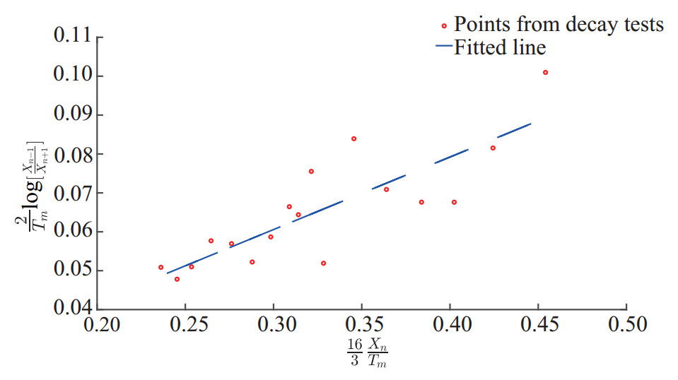Figure  23  Illustration of how the damping coefficients p₁ and p₂ (see Eq. (3)) are obtained form the decay test

Download: Full-Size Img

One should note that the obtained damping coefficients might not be 100% correct. In fact as explained in Faltinsen (1993), it is difficult and in some cases impossible to determine the straight line from the decay tests. It means we can not find one p₁ and p₂ value that is valid for the total decay time. So some calibration on the obtained values might be needed. After obtaining the values and multipying them with the ship mass and added inertia, the following damping coefficients are extracted:

Now we use these damping terms in the potential-based seakeeping solver and try to simulate the C529 and C541 roll decay cases. The comparison of the obtained results for both cases are shown in Figures 24 and 25.

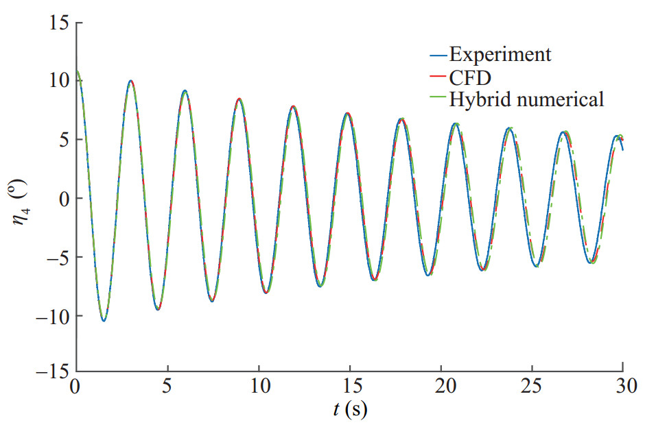Figure  24  Comparison of roll decay of experimental results and potential solver and CFD results for case C529

Download: Full-Size Img

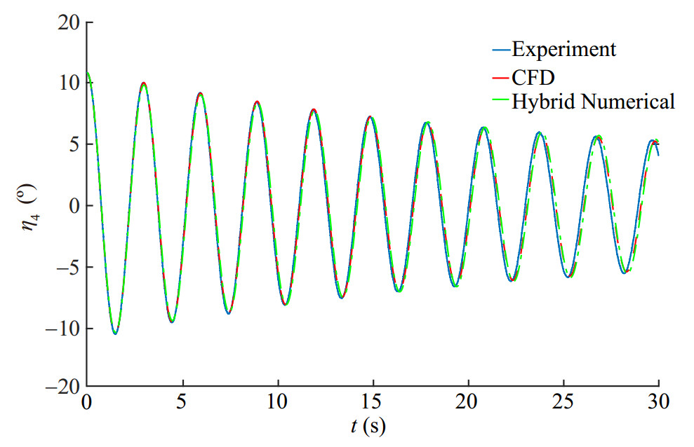Figure  25  Comparison of roll decay of experimental results and potential solver and CFD results for case C541

Download: Full-Size Img

It is shown that the obtained damping values used in the potential-based solver could reproduce the roll decays perfectly. However it can be seen that the difference in the case C541 is slightly higher than the case C529 which was predicted due to the larger roll amplitudes. As it was stated before, the extracted non linear roll damping is assumed to be constant with respect to the roll amplitude which is not exactly true. This might have effects in the larger error in case C541. The agreement is generally acceptable and it can ensure us about incorporating the correct viscous damping in the simulations. Now the obtained damping values are used in the potential-based solver for further seakeeping analyses in the next section.

5.2   Results in parametric rolling analysis

Now by having the correct roll damping level of the system, we can start simulating the motions in the waves. We decided to do the simulations for the described vessel in the vicinity of the parametric resonance in the roll motion area. This area is picked because the experimental results are available from Ghamari (2019). Another reason for picking this area is that the parametric rolling is highly dependent in the damping level and the accuracy of the prescribed method in this paper could be tested by this analysis perfectly. The selected study cases for this part is shown in Table 9. These cases lie in the middle of the instability area where the parametric rolling are most likely to occur.

The correct formulation for a general ship motion (including the transient part), should include the convolution integral in the radiation forces. The radiation loads computed in the frequency domain could be transferred to the time domain by Fourier transformation (as suggested by Cummins formulation Cummins (1962)). Then the complete 6-DOF time domain formulation for the body motions can be written as:

where M_jk is the mass matrix, A_jk(U, ∞) is the added mass coefficient in the infinite frequency, B_jk(U, ∞) is the damping coefficient in the infinite frequency, C_jk^rad is the radiation restoring (comes up in the Cummins formulation Ghamari (2019)), K_jk is the retardation function, η_k and $ {{{\dot \eta }_k}}$ and $ {{{\ddot \eta }_k}}$ are the motion, velocity and acceleration in the kth mode, the F_j^diff is the diffraction force, F_j^FK is the non-linear Froude-Krylov force, Fjrest is the non-linear hydrostatic restoring force, F_j^grav is the ship weight and F_j^others are the other forces that might be imposed to the ship, like the mooring line forces and so on. All of them are expressed in terms of their jth component. One should note that, strictly speaking Cummin's approach Cummins (1962), is valid within linear theory, i. e. for linear non steady-state problems. Researchers have stretched this to the limits including on the right-hand-side nonlinear loads and keeping the assumptions of linearity for the radiation and diffraction loads. The same strategy has been used here.

The system of the mentioned equations is solved here using a time integration algorithm based on the Rung-Kutta fourth order (RK4) method with constant time steps, 0.005 times of the wave period. More information about this solver and the setup of this study could be found in detail in Ghamari (2019). The roll damping in this system is set to zero and the extracted roll damping which is a key parameter in this analysis are incorporated in this solver. The obtained experimental and numerical results for the roll-motion amplitude in nearly steady-state conditions in all studied cases are shown in Table 10.

As it can be seen from the comparison of the results, in all 9 cases, PR are captured numerically. The results are the same in terms of occurrence of PR and the roll amplitudes also show an acceptable agreement. It should be noted that due to the highly nonlinear nature of the PR phenomena, we can not expect higher agreement between numerical and experimental results in terms of roll amplitude. There are many nonlinear phenomenon like, bow flare and stern slamming and also water on deck that are not modeled in the numerical simulations correctly. These effects are investigated in detail in Ghamari (2019). As a sample case, the comparison of the numerical and experimental results of the roll motion for the case C457 is shown in Figure 26.

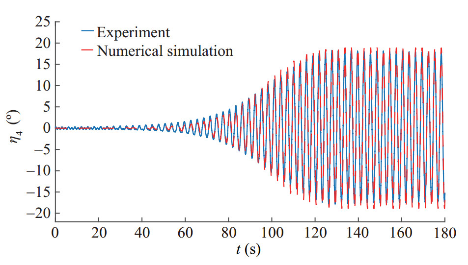Figure  26  Comparison of experimental and numerical roll motion for case C457

Download: Full-Size Img

As it could be seen in the figure, the results are in a good agreement. In the roll motion, the build-up phase and the steady state amplitudes show satisfactory agreement. But it should be borne in mind that the important parameter in the PR analysis is its occurrence and the steady-state roll amplitude. In a practical case, the build-up phase of the roll motion would also matter to characterize the time scale for PR to reach critical roll angles. However, in the experiments, this build-up phase is much affected by the used set up which might not be exactly the same in the numerical simulation setup. There are numerical and experimental error sources that might have influenced the results. In the experiments, the heave and pitch motions are not very regularly oscillating even in the steady-state phase for all cases. That is partly due to the incident waves which are not perfectly regular because of reflection of waves from the tank walls. There are many non-linearities connected to the breaking waves at the ship bow observed for many cases (especially for cases with forward speed), to the bottom and bow flare slamming and even to water on deck in some cases. Small misalignments from the head sea waves in the experiments might also have some influences. The asymmetric cables in port and starboard are also important. Besides, in the numerical side, the interaction between the local steady flow and unsteady flow, for the advancing vessel, is ignored in the numerical solver. It might have some effects on the results especially for this ship, which is not slender. Furthermore, the local wave elevation (radiation and diffraction waves) is not considered in the wetted surface of the body in time.

6   Conclusion

The main purpose of this paper was to present the RANS based CFD capabilities in capturing the roll damping of a vessel. A gap in the literature for the potential-based seakeeping solver was identified as viscous roll damping. It is clear that due to the limited computational resources and also time-consuming computations in the CFD-based codes, it is not possible to use them for 6-DOF seakeeping simulations. On the other hand, the potential-based solvers are not capable of estimating the viscous part of the roll damping. The only solution is to use the experimental results or the numerical results by the CFD-based codes for the roll decacy tests. Since the experimental results are not always available for all vessels and it might be so expensive, the CFDbased codes might be a practical alternative. In this paper, the results of the roll decay tests for couple of cases was shown and compared with the experimental ones. The agreement was good and it showed we could use them for extracting the viscous roll damping. Then, we used the extracted roll dampings and incorporate them in the potential seakeeping solver. we analyzed 9 cases which were in the parametric resonance instability ares. The comparison of the experimental and obtained results show a satisfactory agreement. This combination of CFD codes for extracting the viscous damping and potential based seakeeping solver for seakeeping analysis, will ensure the correct level of roll damping level. It also will use the advantage of the potential seakeeping solver which is the low computational time. This efficient and accurate combination could also be used in the design stage when many simulations are needed for optimization purposes.