1   Introduction

Free surface water wave scattering problems involving various kind of structures play an important role in science and engineering. Thin vertical barriers are one such structure that attracted lot of attention due to their potential in developing rich mathematical solution methods to the associated boundary value problems. Dean (1945) derived analytical solution of the two-dimensional normally incident water wave problem with a submerged thin vertical rigid barrier by using the complex variable technique. Then, using integral equation procedure, Ursell (1947) studied water wave scattering problem involving a surface piercing rigid barrier. Scattering of gravity waves by a vertical barrier with finite number of gaps in it was discussed by Lewin (1963), Mei (1966) and Evans (1970). Lewin (1963) and Mei (1966) solved the problem by converting the original problem into a Riemann-Hilbert problem. Evans (1970) used the method of complex variables to obtain the solution of the problem. Mandal and Chakrabarti (2000) proposed various solution methods to obtain the solutions of the wave scattering problems involving different rigid barrier configurations.

Later, porous barriers gained attention due to its reflection and dissipative characteristics. Chwang (1983) introduced porous wave maker theory by involving resistance effects. Then, the condition on the porous barrier has been modified by including inertial effects as well (Yu and Chwang 1994). Further, flexible breakwaters attracted lot more attention due to their structural flexibility. These kind of breakwaters are used in deep sea activities. Incident wave interaction on a flexible barrier that is hinged at the bottom of the sea and moored at the surface was analyzed by Lee and Chen (1990). Also, Williams et al. (1991) investigated flexible floating breakwater that was anchored to the sea floor with a buoy at the free surface.

Kim and Kee (1996) and Cho and Kim (1998) have studied wave interaction with a horizontal tensioned flexible membrane by utilizing the eigenfunction expansion method. Selvan and Behera (2020) have used the same method to handle the effect of a floating circular porous elastic membrane on surface gravity waves. Later, Cho and Kim (2000) discussed interaction of incident waves with a horizontal porous flexible membrane by using the multi-domain boundary element method. Yip et al. (2001)have investigated the oblique wave scattering problem involving finite number of floating membranes in finite water depth. Then, Suresh Kumar et al. (2007) have analysed wave scattering by a vertical flexible porous membrane in a two-layer fluid of finite depth, using an orthogonality relation along with the least-square approximation. Karmakar and Guedes Soares (2012) have analyzed the performance of the multiple vertical surface-piercing porous membrane barriers in water of finite depth by applying the least-square approximation method. Mandal et al. (2016) studied oblique wave scattering problem involving the multiple flexible porous barriers in a two-layer fluid of finite depth. Using eigenfunction expansion method, Koley and Sahoo (2017) have investigated the oblique wave scattering problem involving different configurations of a vertical flexible porous membrane.

A single term Galerkin's method has been used by Evans and Morris (1972) to handle obliquely incident waves on a surface piercing rigid barrier and they found closed upper and lower bounds for the scattering quantities. Also, scattering of oblique incident surface waves by a finite length thin submerged vertical plate as well as a complete barrier with a gap in it has been handled by Mandal and Das (1996) and Das et al.(2018a, 2019). They used one or two term Galerkin method to find the scattering quantities analytically. Further, Galerkin method with many terms is utilized to solve oblique scattering problem involving a partially immersed and a submerged solid barrier by Das et al. (2018b).

A flexible porous tensioned membrane is considered here with all four type of configurations such as partially immersed, submerged barrier extending infinitely downwards, submerged barrier with a finite length and a complete membrane with a gap in it. Free surface waves incident obliquely on the barrier from either side are considered. This defines two solution velocity potentials for the original problem. The upper-half plane problems for the two velocity potentials are reduced to problems in a quarter-plane. These quarter plane problems are connected with auxiliary potentials through a couple of integral relations. Then, the auxiliary potentials are handled by the Galerkin's method with one or multi-term approximation.Further, lower and upper bounds for the scattering quantities are obtained. Formulation of the boundary value problem and its solution method is described in Section 2. In Section 3, numerical results are discussed for each of the barrier configuration by choosing a suitable weight function in the approximation. Finally, few conclusions are drawn in Section 4.

2   Mathematical formulation and method of solution

A mixed boundary value problem is considered in the Cartesian coordinate system (x, y, z) with the positive y-ax-is measured vertically downwards and the horizontal xz-plane is the undisturbed free surface. The fluid is occupied in the domain y >0 and −∞ < x, z < ∞. The vertical porous membrane is placed in the fluid region at x=0, y∈B and −∞ < z < ∞ in which B takes one of the following: (0, a), (b, ∞), (0, a) ∪(b, ∞) and (a, b). The fluid is considered to be inviscid, incompressible and the flow is in irrotational motion. Incident surface waves come from x=∞ and make an angle β with the xy- plane. Under the assumptions of the linearised water wave theory, time-harmonic fluid motion is described by the velocity potential Re{ϕ1 (x, y)e^ipzee^{− iωt}}, where p=Ksinβ, K=ω²/g in which ω is frequency of the incident wave, g is the acceleration of gravity and t is time.The same wave motion is also described, when the incident waves come from x=−∞ and make an angle π-β with the xy- plane, by the velocity potential Re{ϕ₂ (x, y)e^ipze^iωt}. Then, the spacial velocity potentials ϕ_j(x, y), j=1, 2 satisfy

The free surface boundary condition is

In addition, ϕ_j(x, y), j=1, 2 satisfy the conditions

and

where r is the local radius from the edge point of the barrier. The schematic diagram for the oblique wave scattering problem is shown in Figure 1.

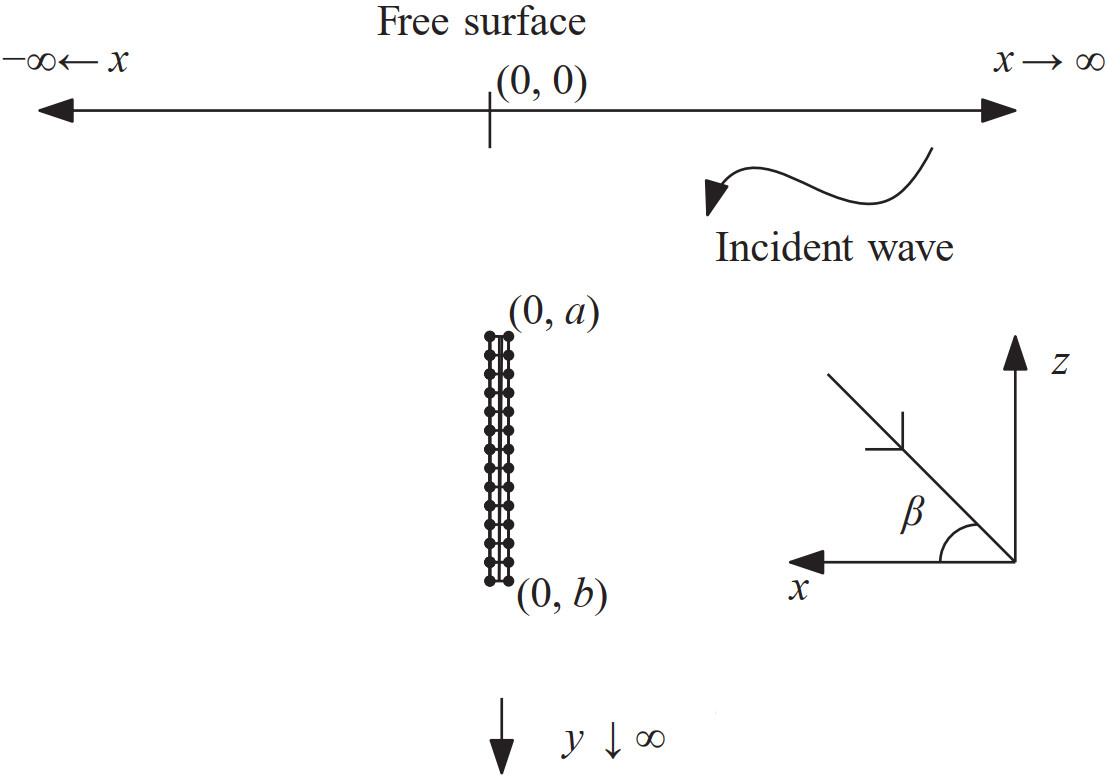Figure  1  Free surface with submerged flexible porous membrane

Download: Full-Size Img

The displacement of the horizontally oscillating membrane is represented as

where ν_j(y) is the deflection amplitude of the membrane.

Assume that the absolute value of the deflection amplitude is small as compared to the incident wave length. The boundary condition on the flexible porous membrane (Yu and Chwang 1994) is given by

where Γ=Γ₁+i Γ₂ is the non-dimensional complex porous effect parameter in which Γ₁ is the resistance effect and Γ₂ is the inertial effect.

The fluid flow is continuous in the gap x=0, y ∈ B =(0, ∞) \ B. That is,

The radiating conditions are described as

where ϕ⁰(−x, y)=e^{−i K x cosβ−K y} is the incident wave potential and R, T are amplitudes of the reflected, transmitted waves. Also, the deflection amplitude ν_j(y), j=1, 2 of the membrane satisfies the following condition

In the above, T is tension in the membrane, ρ is the density of water. The membrane frequency parameter may be de‐ fined as $ \alpha=\omega \sqrt{m_{s} / T}$, where m_s=ρ_sd_s is the uniform mass with ρ_s and d_s being the uniform mass density and the thickness of the membrane, respectively.

By utilizing the above equation in Equation (5), the boundary condition on the barrier Equation (5) is obtained as

2.1   Reduction to quarter-plan problems

In view of the continuity of the horizontal velocity of the fluid across x=0, the original velocity potentials ϕ_j, j=1, 2 that are defined in the upper-half plane may be modified into a new potential functions ψ_j, j=1, 2 in the quarterplane. This is done by choosing (Lamb 1932)

The potential functions ψ_j defined in the domain (−1)^j+1 x > 0, j=1, 2 satisfy Equations (1)‒(4). By applying Equation (7) to the Equation (6), the boundary condition on the barrier becomes

In addition, the boundary condition in the gap and the radiation condition become

and

ψ_j(x, y)➝(R − 1)ϕ⁰ (x, y) as (−1)^jx➝ − ∞, j = 1, 2

with a note that T=1−R.

2.2   Connection between wave potentials

A well defined connection, similar to the one in Ashok et al. (2020), between the flexible porous wave potential ψ_j (x, y), j=1, 2 and the auxiliary potential χ_j(x, y), j=1, 2 is introduced as

where $ C_{j}(u, y)=\phi^{0}(u, y)+\phi^{0}(-u, y)+\sum_{m=1}^{2} \psi_{\mathrm{m}}\left((-1)^{j+m} u, y\right)$.

The auxiliary potential functions χ_j(x, y), j=1, 2 satisfy Equations (1)‒(4). By differentiating the connection Equation (10), one obtains

where the variable suffix denotes derivative. By setting x=0 in Equation (11) and by applying the equation Equation (8), it may be obtained that

Also, by setting x=0 and by using the equation Equation (9) in the connection Equation (10), one finds the condition as given by

Further, the radiation condition for χ_j(x, y), j=1, 2 may be specified as

where R_j and T_j are constants. By applying the far-field behaviour in each term of the differential form of the connection Equation (11), a pair of relations is obtained as

and

Thus, the problem for the wave potential ψ_j(x, y) with j=1, 2 has been decomposed into two solvable auxiliary potential problems with the aid of the connection Equation (10). Hence, the solution of the auxiliary potential ψ_j(x, y) may be found in terms of the wave potentials χ_j(x, y) as in Ashok et al. (2020). The approximate solution of the wave potentials χ_j(x, y) j=1, 2 is obtained by the Galekin approximation method which in turn helps to find the estimated value of the reflection coefficient |R|.

2.3   Galerkin method

The general solution of the potential function χ₁(x, y) satisfying Equations (1) ‒ (3) and Equation (14) is given by (Manam et al. 2006)

where R₁, T₁ are unknown constants, A(γ) is an unknown function, $ B(\gamma, y)=\gamma \cos \gamma y-K \sin \gamma y \text { and } \gamma_{1}=\sqrt{\gamma^{2}+p^{2}}$.

Let

By utilizing the general solution Equation (17) in the above functions g(y) and h(y), it may be obtained that

and

Then, the Havelock's inversion theorem (Havelock 1929) is applied to the above pair of equations to get

and

By substituting A(γ) from Equations (21) and (23) in the equations Equations (19) and (18) and then using the conditions (12) and (13), it may be obtained that

and

where

and

Now, by defining the functions

and then, by making use of G(u) and H(u) in Equation (24) and Equation (25), one obtains that

and

Then, the Equations (20) and (22) are modified as

and

where

The Equation (15) and Equation (16) are used in the above to find

In a similar manner, the same estimation of the constant F in terms of the reflection amplitude R can be obtained for the problem of the auxiliary potential function χ₂(x, y), by the aid of the Equations (15) and (16).

2.4   Bounds for F

Multi-term Galerkin approximation method is used to find the functions G(u) and H(u) in the Equations (26) and (27) (Das et al. 2018b). We first define the symmetric and linear inner products as

Then, we define a pair of operators C and D as

Note that the operators C and D are linear, positive semidefinite and self-adjoint. To obtain the function G(u) in Equation (26), we take the multi-term Galerkin approximation as given by

where g_n(y), n=0, 1, …, N may be chosen appropriately for a particular barrier position.

By making use of Equation (31) in Equation (26), and multiplying the function g_m(y) before integrating over B, we get the linear system of equations

where

The constants a_n, n=0, 1, …, N are found by solving the above system of equations. By following Evans and Morris(1972), it is seen that

By substituting the equation Equation (28) in the above inequality, one obtains that

where

Further, the function H(u) in Equation (27) can be found by considering the multi-term Galerkin approximation

where h_n(y), n=0, 1, …, N is chosen appropriately for a particular barrier problem. By substituting Equation (34) in Equation (27) and multiplying the function h_m(y) before integrating over B, we obtain the linear system of equations for the unknowns b_n, n=0, 1, …, N as given by

where

Again, by following Evans and Morris (1972), it is seen that

By utilizing the Equation (29) in the above inequality, with the use of the far-field Equations (15) and (16), it is obtained that

where

By modifying the relation Equation (30), the reflection coefficient is obtained as

where F_l≤F≤F_u. The upper and lower bounds for the reflection coefficient may now be found as

where

and

The upper bound R_u is computed first and then use it in the Equation (35) to estimate the lower bound F_u which is matched with the lower bound F_l. In the computation, it is found that these bounds for F are numerically matched up to few decimals.

3   Numerical results for various barrier positions

The dimensionless membrane mass and tension parameters $ \delta_{1}=\frac{m_{s}}{\rho l}$ and $ \varepsilon_{1}=\frac{T}{\rho g l^{2}}$ are used in the numerical computation while fixing the value of the length of the porous membrane l=2 m and the density of the sea water ρ =1 025 kg/m³. Also, the membrane parameter value α =0.062 46 is obtained by fixing the incident wave frequency ω=1.75 s⁻¹, δ₁=0.01 and ε₁= 0.4. Energy identity |E|=|R|²+|T|²=1 is verified throughout the computation for the impermeable membrane barrier (Γ =0). The porous membrane barrier becomes the solid barrier when Γ=0 and α=0. It is seen that the reflection curves are matching with the ones in already published works when Γ=0 and α=0 are fixed for all the four barrier configurations.

3.1   Surface piercing finite membrane

In this case, the position and the gap are at B=(0, a) and B= (a, ∞), respectively. The function G(y) has been taken (Das et al. 2018b) as

where a_n, n=0, 1, …, N are unknown constants and

The nature of the edge behaviour of the membrane is considered for taking the weight function g_n(y), n=0, 1, …, N. Now, we calculate the analytic results for a two-term Galerkin approximation (N=1). Consider g₀(y) and g₁(y). Then, by solving the system Equation (32) to obtain F_l as

where

and G_i0=a K_i(2Ka), i=0, 1 in which K_i(2Ka), i=0, 1 are modified Bessel functions. It is observed that B₀₁=B₁₀ from symmetry of the kernel of the integral equations. Further, the constants A₀₀, A₀₁ and A₁₁ are known as

and

where

Also, H(y) can be taken as

where b_n, n=0, 1, …, N are unknown constants. The weight functions h_n(y), n=0, 1, …, N are given by

The same procedure is applied for the two-term Galerkin approximation, as mentioned above, to obtain the upper bound F_u. It is numerically verified that both the upper and lower bounds are matching up to few decimals to estimate the value of the reflection coefficient |R|.

The reflection coefficient |R| and the total energy |E| =|R|²+|T|² are calculated against the angle of incidence β. In Figures 2 and 3, estimation of the reflection coefficient |R| and the total energy |E| are depicted versus the angle of incidence β for various values of the wavenumber Ka with the membrane frequency parameter α =0.062 46 for both cases of porous as well as impermeable membranes. It may be observed, from Figures 2 and 3, that enhanced reflection and enhanced dissipation occur at smaller incident angles for shorter waves. The angle at which wave reflection gets its resonant peak increases with a decrease in the incident wave number. The reflection peak increases as length of the barrier increases, this is due to larger barrier reflect more waves. Also, complete reflection occurs at these incident angles in the case of the impermeable membrane.

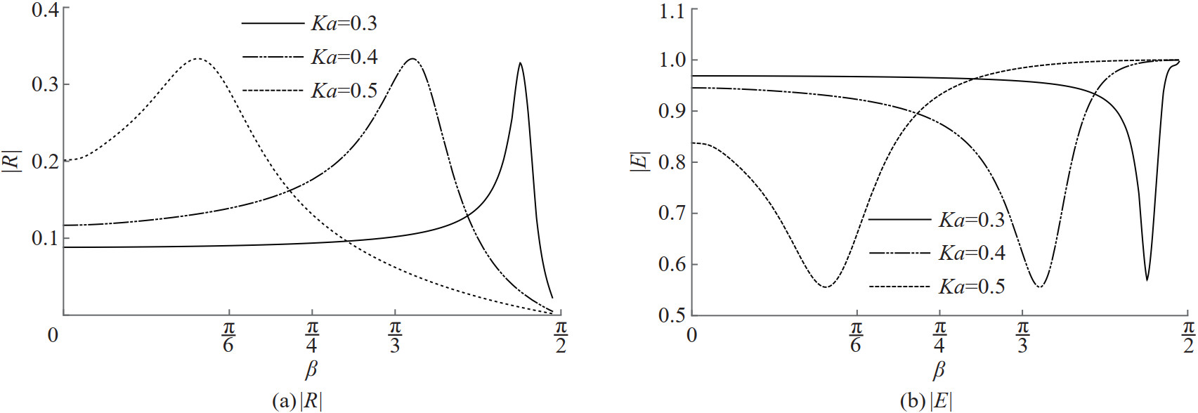Figure  2  Graph of |R| and |E| versus β for different values of Ka with Γ=1 and α=0.062 46

Download: Full-Size Img

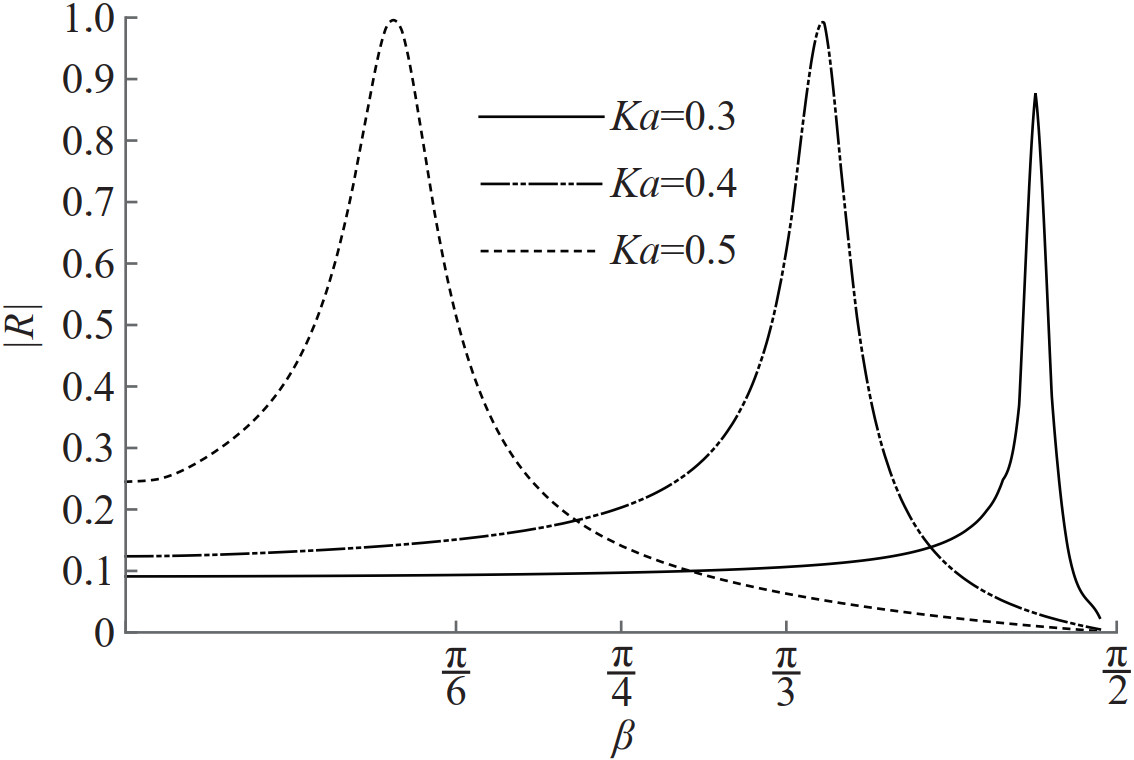Figure  3  Graph of |R| versus β for different values of Ka with Γ=0 and α=0.062 46

Download: Full-Size Img

Reflection and energy curves are plotted against the angle of incidence for various values of the membrane frequency parameter α in Figures 4 and 5. For smaller values of α, there is neither enhanced reflection nor enhanced energy loss for all angles of wave incidence. Reflection decreases gradually with an increase in the angle of incidence for all values of the membrane frequency parameter. For smaller values of incidence, reflection is higher for the porous membranes with lesser tension. Also, mass of the membrane barrier increases when the reflection increases for shorter waves. This is because of barrier with higher mass reflect better. As expected, energy dissipation is higher for membranes with lower tension at smaller angles of wave incidence. However, enhanced reflection and total wave energy dissipation occur for porous membranes. Reflection or energy dissipation peaks happen at larger incident angles with a decrease in the tension of the porous membrane.

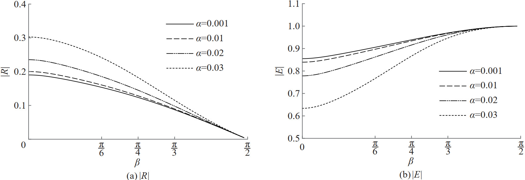Figure  4  Graph of |R| and |E| versus θ for different values of α with Γ=1 and Ka=0.4

Download: Full-Size Img

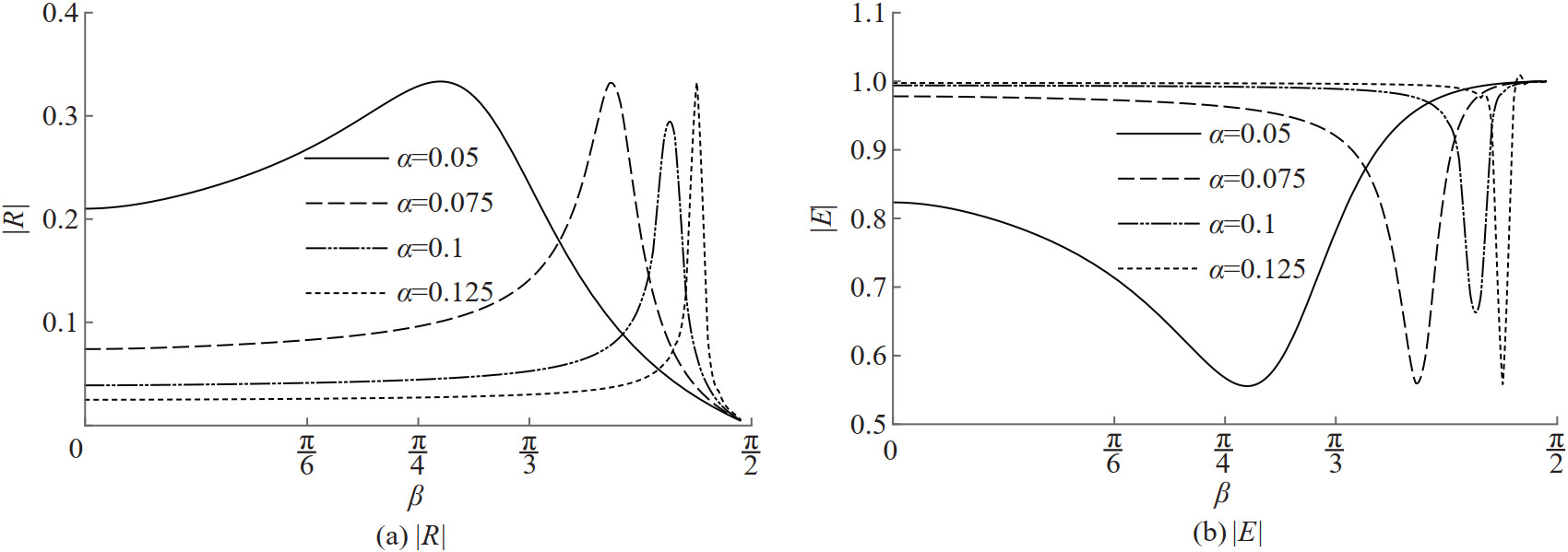Figure  5  Graph of |R| and |E| versus β for different values of α with Γ=1 and Ka=0.4

Download: Full-Size Img

Reflection and energy curves are depicted against the angle of incidence β for different values of the porous effect parameter Γ when the values of α =0.062 46 and Ka=0.4 are fixed in Figure 6. It is seen from Figure 6(a) that reflection in general is better for small incident angles when both the resistance and the inertial effects are present in the porous barrier. Further, all the reflection curves have peaks that are due to the flexible nature of the barrier and they occur within 50° to 75°. Also, enhanced reflection is evidently complete for the impermeable membrane. Enhancement of the energy dissipation may be seen from Figure 6(b) around a particular angle of wave incidence forall the values of the porous effect parameter. In Figure 7, reflection and energy curves are plotted against the angle of incidence β for various values of the porous effect parameter Γ when α=0 and Ka=0.4. Overall reflection significantly decreases again for the resistance as well as the inertial effects for small angles of wave incidence on the porous solid barrier. Figure 7(a) also shows that porosity alone will not cause enhanced reflection by the barrier since there is no evidence of the enhanced reflection in the absence of flexibility in the barrier. Also, as seen from Figure 7(b), en‐ergy dissipation is evidently caused mainly from the inertial effects of the porous barrier. The smaller reflection is noted for the porous membrane barrier due to the fact that the porous barrier allows the water to pass through it.

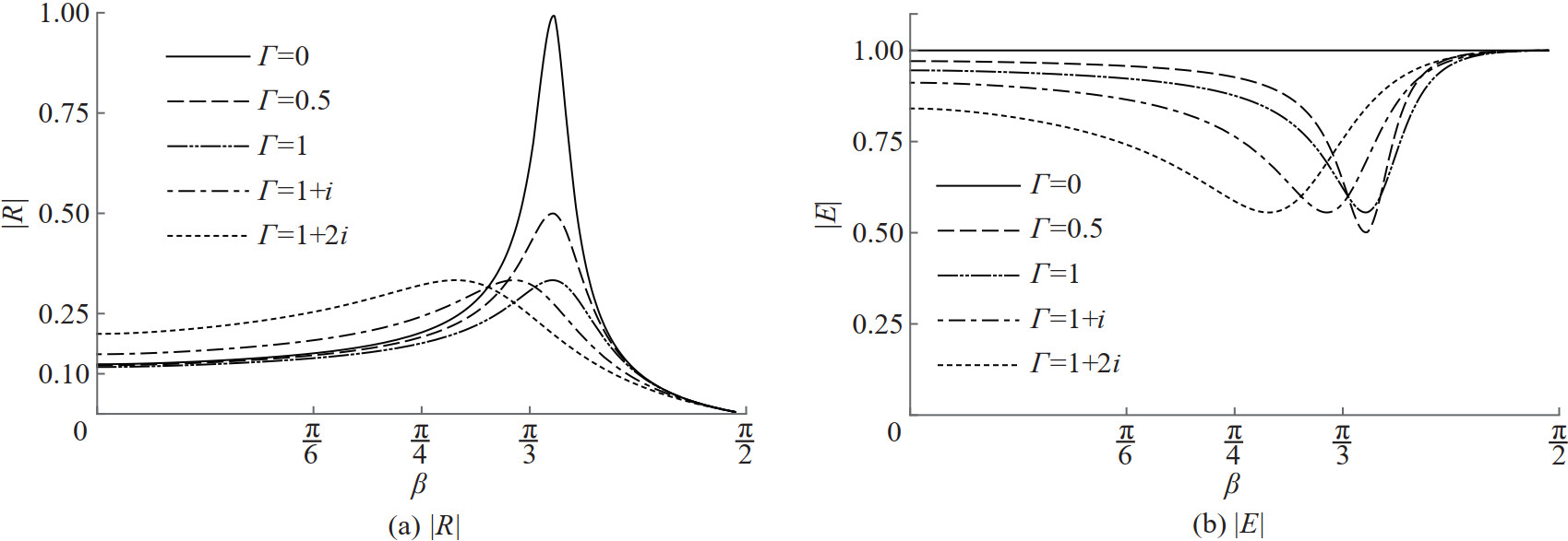Figure  6  Graph of |R| and |E| versus β for different values of Γ with α=0.062 46 and Ka=0.4

Download: Full-Size Img

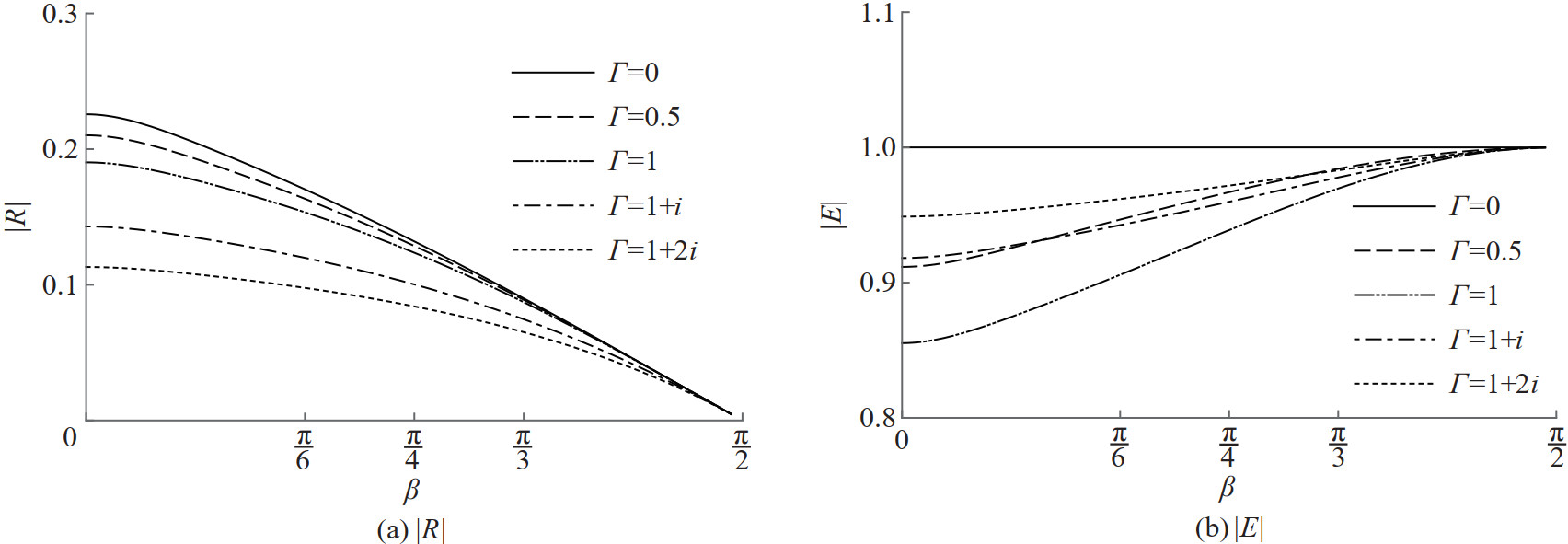Figure  7  Graph of |R| and |E| versus β for different values of Γ with α=0 and Ka=0.4

Download: Full-Size Img

3.2   Submerged membrane of infinite length

The membrane position and gap are at B=(b, ∞) and B= (0, b) respectively. Again, the multi-term Galerkin approximation is used and G(y) (Das et al. 2018b) is set as

where a_n, n=0, 1, …, N are unknowns to be determined and the weight functions g_n(y), n=0, 1, …, N are

Again, the nature of the edge behaviour of the membrane is considered for choosing the weight function g_n(y), n=0, 1, …, N. Then, two-term Galerkin approximation (N=1) is used to solve the linear system Equations (32). The lower bound F_l can be obtained as F_l=a₀ G₀₀+a₁G₁₀, where

In the above, the constants A₀₀, A₀₁ and A₁₁ are

and

where

Now, H(y) can be taken as

where b_n, n=0, 1, …, N are unknown constants. The weight functions h_n(y), n=0, 1, …, N are given by

Moreover, the upper bound F_u is obtained by using the same procedure explained in the two-term Galerkin approximation method.

The reflection coefficient |R| and the total energy |E| =|R|²+|T|² are evaluated against the wavenumber Kb and the angle of incidence β for the submerged barrier extending infinitely downwards.

In Figure 8, numerical estimation of the reflection coefficient |R| and the total energy |E| are plotted against the angle of wave incidence β for different values of the wavenumber Kb when Γ=1 and α=0.062 46. These curves are also shown in Figure 9 for the non porous membrane with the same flexibility. It is observed from Figure 8 that the reflection and the energy dissipation curves have resonant enhancement for all the incident wave numbers. Since the present barrier is the complementary nature of the previous case in the subsection 3.1, the resonant peaks at which enhanced reflection occurs move from lower to higher wave incident angles when the incident waves on the barrier become longer to shorter. This is exactly opposite to the results of the previous complementary case. Similar observation can be made for the energy dissipation curves with the change in the incident wavenumber. Flexibility alone causes the total reflection from the submerged non-porous membrane as seen from Figure 9. Thus, longer waves should incident the membrane by higher oblique angles to get better or complete reflection while shorter waves could incident the membrane by smaller oblique angles for a similar enhanced reflection.

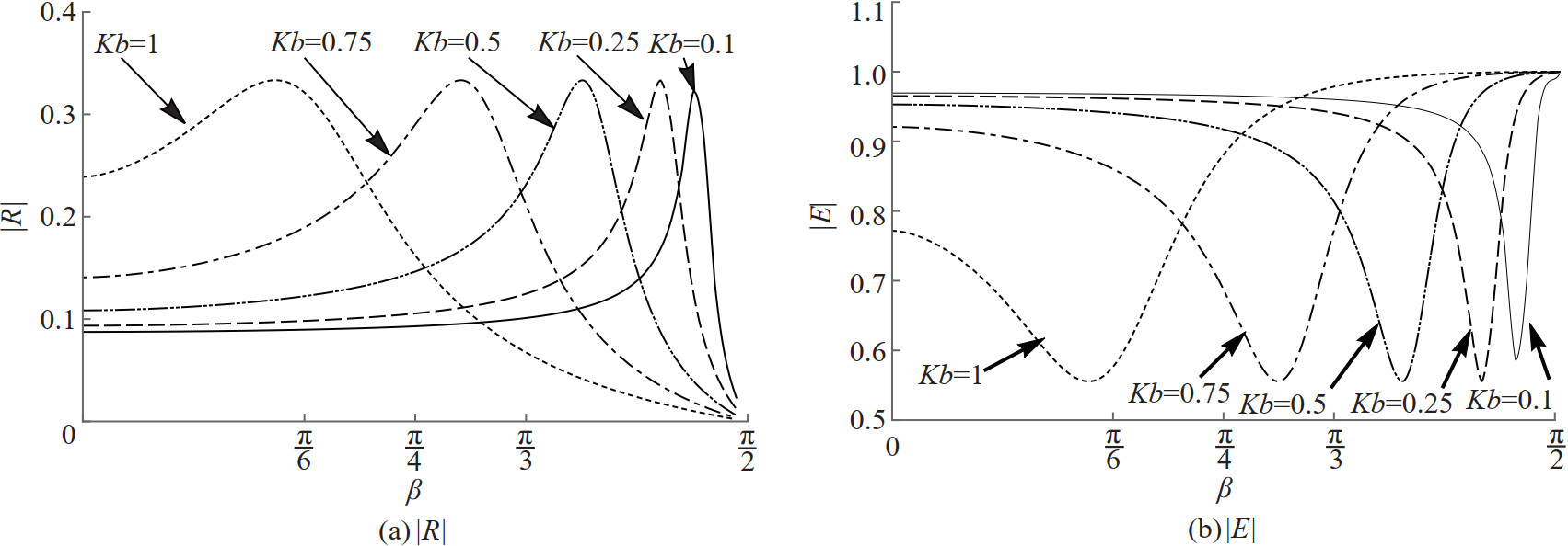Figure  8  Graph of |R| and |E| versus β for different values of K b with Γ=1 and α=0.062 46

Download: Full-Size Img

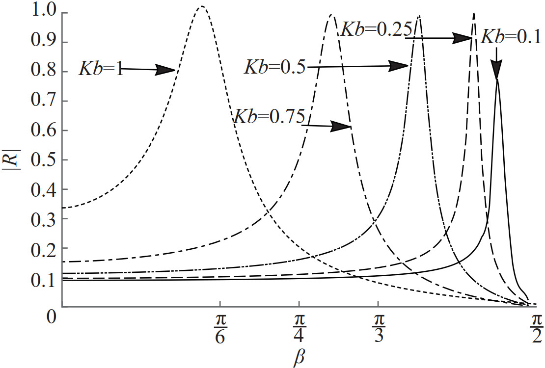Figure  9  Graph of |R| versus β for different values of Kb with Γ=0 and α=0.062 46

Download: Full-Size Img

In Figure 10, reflection and energy curves are depicted against the angle of wave incidence for various membrane frequency parameter values when the wavenumber Kb=0.4 and Γ=1 are fixed.The reflection peaks move towards higher oblique wave angles as the membrane frequency parameter increases. Similar behaviour is seen in the surface piercing membrane case as well. This shows that only flexibility nature of the barrier, not a type of the barrier, causes the enhanced reflection. The reflection and energy curves are also plotted against the wavenumber for different membrane frequency parameter values when the angle of oblique incidence β=30° and Γ=1 are fixed in Figure 11. However, reflection peaks move towards shorter incident waves as the membrane frequency parameter increases. This suggests longer waves must incident on a high tensioned membrane and shorter waves must incident on a low tensioned membrane to get better resonant reflection. Reflection peak is attained for shorter and moderate waves for smaller mass of the membrane barrier. Similar observations can also be made from the energy curves in Figure 11.

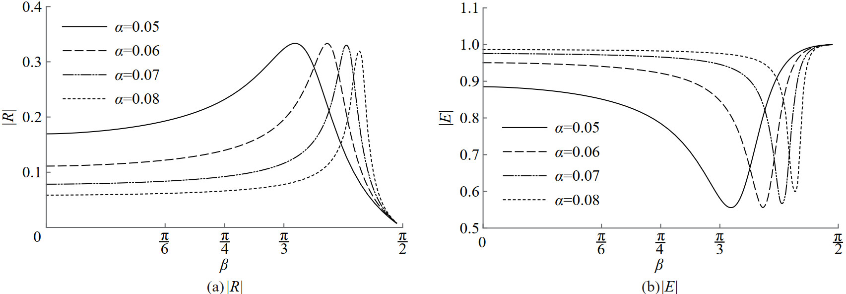Figure  10  Graph of |R| and |E| versus β for different values of α with Γ=1 and Kb=0.4

Download: Full-Size Img

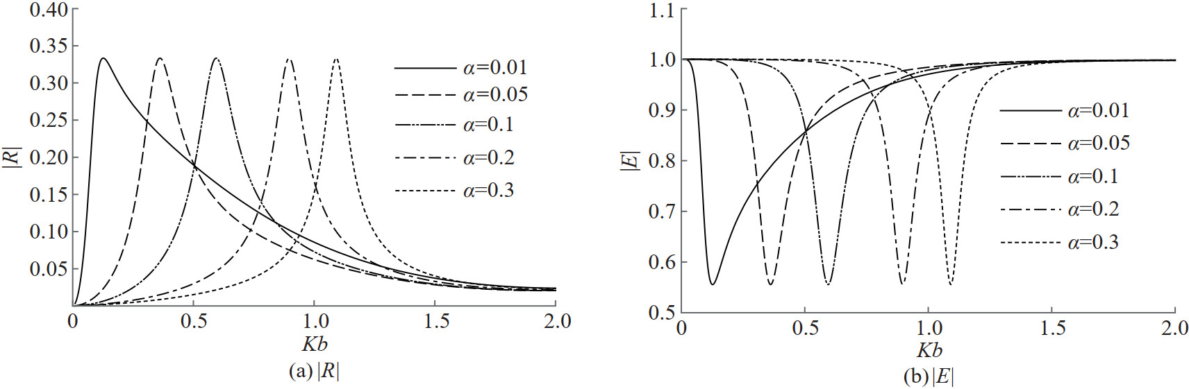Figure  11  Graph of |R| and |E| versus Kb for different values of α with Γ=1 and β=30°

Download: Full-Size Img

Reflection and energy curves are also depicted against the angle of incidence for various porous effect parameter values when the wavenumber Kb=0.4 and α=0.062 46 are fixed in Figure 12. By comparing these curves with the ones in Figure 6, it may be concluded that the reflection and the energy dissipation is mostly caused by the flexible nature of the membrane. Enhanced reflection becomes a complete one for the impermeable barrier at a particular incident wave angle as observed in the case of surface piercing membrane barrier. Figure 13 shows reflection and energy curves for the solid porous barrier. They are qualitatively comparable with the ones in Figure 7.

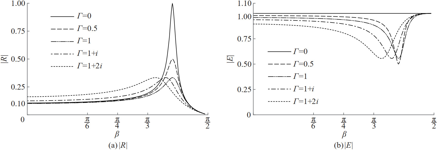Figure  12  Graph of |R| and |E| versus β for different values of Γ with α=0.062 46 and Kb=0.4

Download: Full-Size Img

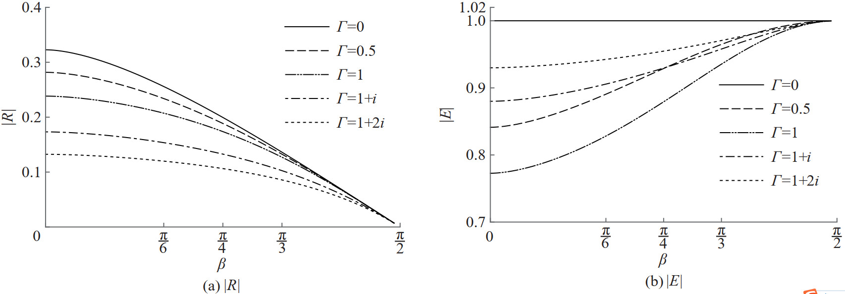Figure  13  Graph of |R| and |E| versus β for different values of Γ with α=0 and Kb=0.4

Download: Full-Size Img

3.3   Submerged membrane of finite length

In this case, the membrane position and the gap are atB=(a, b) and B=(0, a)∪(b, ∞) respectively. The Galerkin approximation for G(y) is specified as $ G(y) \approx \sum_{n=0}^{N} a_{n} g_{n}(y)$, where a_n, n=0, 1, …, N are unknown constants and g_n(y), n=0, 1, …, N are the weight functions. The nature of the edge conditions of the porous membrane is considered to set g_n(y) as

Here, we obtain the analytic results by using a single term Galerkin approximation (N=0). Consider g₀(y). Then, by solving the linear system Equation (32), we obtain a₀=G₀₀/A₀₀. By using a₀ into Equation (33) and get F_l=G₀₀²/A₀₀ where

and

with

Likewise, a single term Galerkin approximation for the function H(y) is specified as

Again, the edge behaviour of the membrane is considered to set h_n(y), n=0, 1, …, N as

Then, the upper bound F_u is obtained by using a single term Galerkin method. Thus, the reflection and the transmission coefficients are attained between two close bounds and the numerical results are obtained for the scattering quantities against various parameters.

The reflection coefficient |R| and the total energy |E| =|R|²+ |T|² are calculated against the non-dimensional wavenumber Kb as well as the angle of incidence β for a submerged barrier of finite length. Numerical estimation of the reflection and the energy curves are plotted against the wavenumber Kb for various $ \mu=\frac{a}{b}$ values when β=30° and Γ=1 are fixed in Figure 14. For the fixed barrier length parameter μ, wave reflection and energy loss reach maximum for waves with a moderate wavelength. The measure of these quantities are remained uniform for moderate to short incident waves. For fixed larger wavenumber, the length of the barrier decreases as reflection decreases. It is due to shorter waves interaction with smaller barriers.

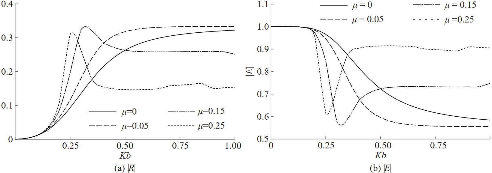Figure  14  Graph of |R| and |E| versus Kb for different values of μ with β=30° and Γ=1

Download: Full-Size Img

In Figures 15 and 16, the reflection coefficient and the total wave energy are depicted against the wavenumber for different values of the membrane frequency parameter when the oblique angle of incidence β=30° is fixed, in both cases of the porous and the non-porous membranes, respectively. Reflection increases in general when the tension in the membrane increases for all membrane lengths. Further, enhanced reflection takes place for a specific smaller length of the membrane due to the flexible nature of the barrier. Both reflection and dissipation of wave energy maintain uniformly high for moderate to longer membranes. Similar observations can be made, from Figure 16, in the case of the impermeable tensioned membrane. However, impermeable membranes with higher tension cause significantly higher reflection in comparison with the porous ones.

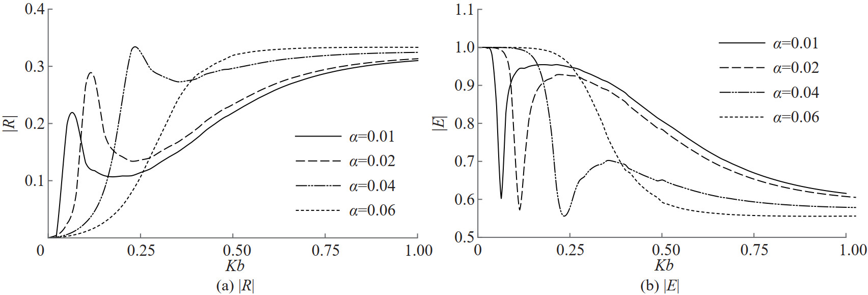Figure  15  Graph of |R| and |E| versus Kb for different values of α with μ=0.05, β=30° and Γ=1

Download: Full-Size Img

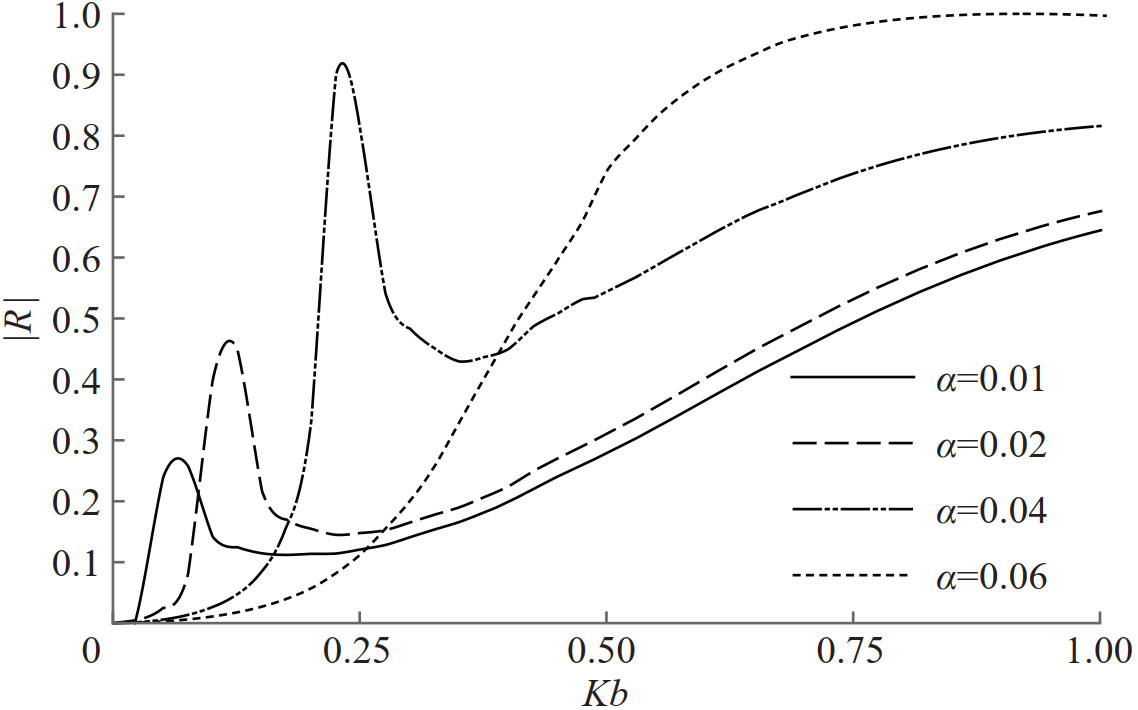Figure  16  Graph of |R| versus Kb for different values of α with μ=0.05, β=30° and Γ=0

Download: Full-Size Img

In Figure 17, the reflection coefficient and the total energy are depicted against the incident wave angle for various Γ values when Kb=0.2 and α =0.062 46 are fixed. From Figure 17, it may be observed that the enhanced reflection and the enhanced energy loss occur in between 30° to 50° and the curves reach minimum in the vicinity of 90°. Again, this is due to the flexible nature of the submerged membrane. Complete reflection is possible at a specific incident wave angle for the impermeable tensioned membrane. This resonant reaction from the barrier is absent when one considers solid porous membrane, as shown in Figure 18. Again, reflection and energy curves for the solid membrane are qualitatively similar to the ones in Figures 7 and 13.

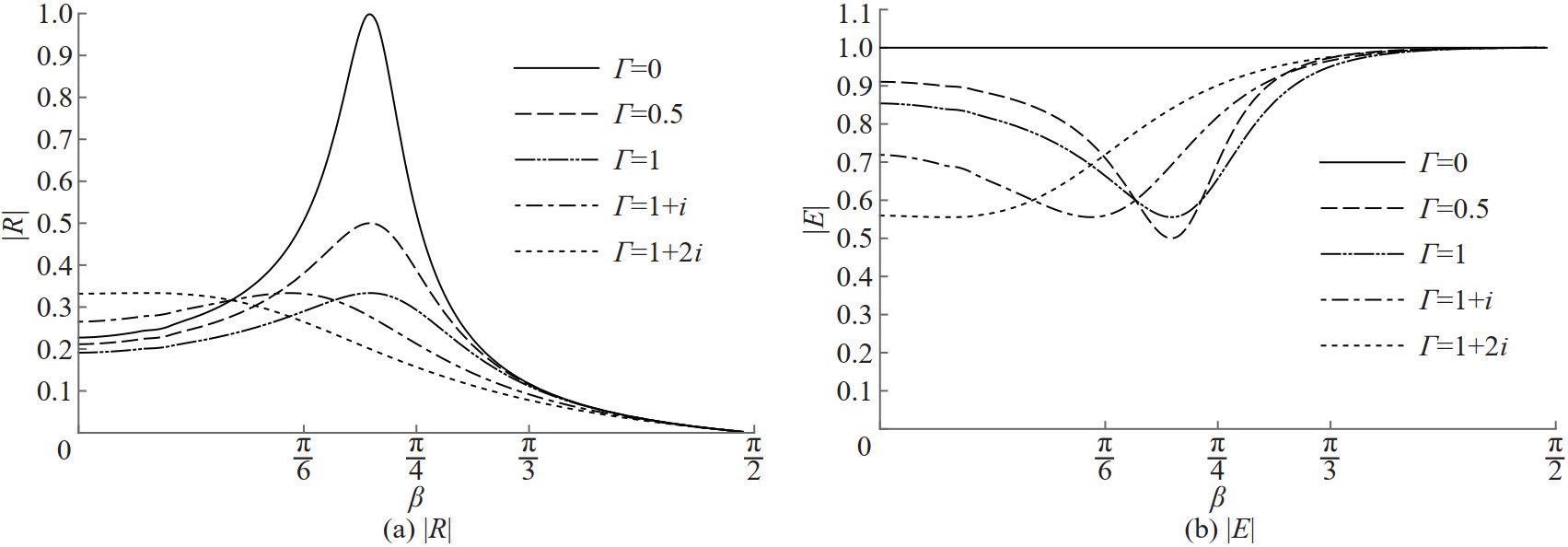Figure  17  Graph of |R| and |E| versus β for different values of Γ with μ=0.5, Kb=0.2 and α=0.062 46

Download: Full-Size Img

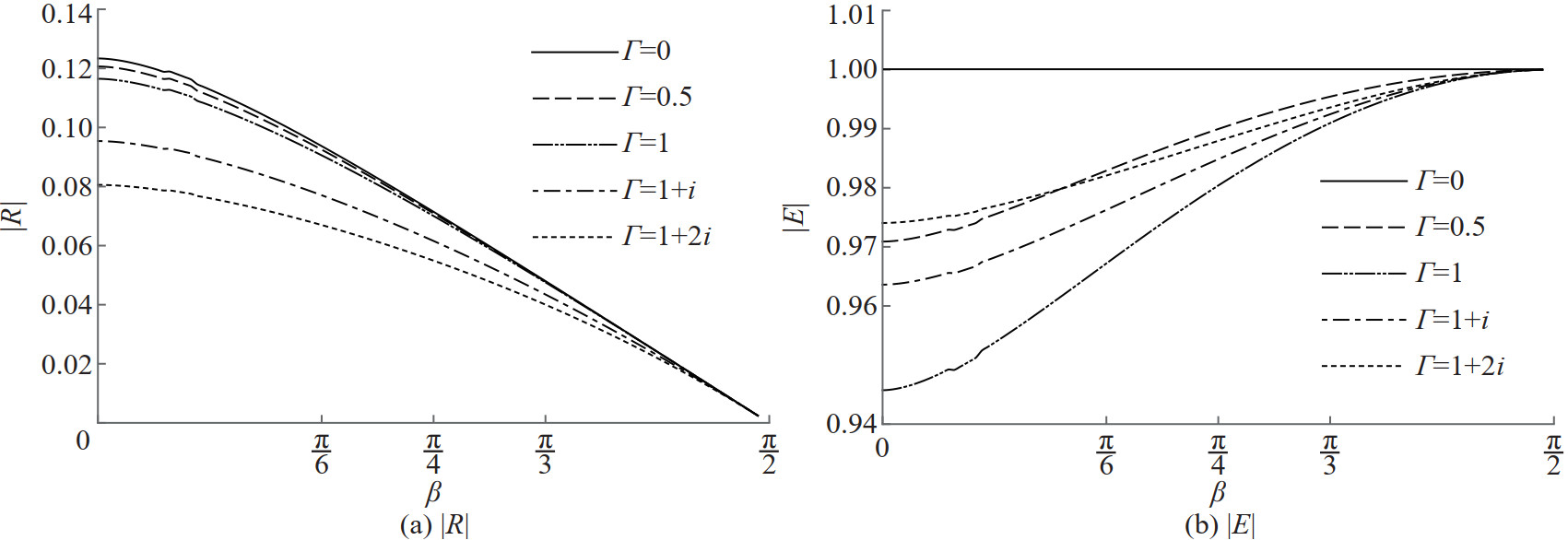Figure  18  Graph of |R| and |E| versus β for different values of Γ with μ=0.5, Kb=0.2 and α=0

Download: Full-Size Img

3.4   Complete membrane with a gap

In this case, the membrane position and the gap are at B= (0, a) ∪ (b, ∞) and B= (a, b), respectively. The multi-term Galerkin approximation for the function G(y) can be taken by

where a_n, n=0, 1, …, N are unknown constants. The edge behaviour of the membrane is considered to set the weight functions g_n(y), n=0, 1, …, N as

Likewise, consider $ H(y) \approx \sum_{n=0}^{N} b_{n} h_{n}(y)$, where b_n, n=0, 1, …, N are unknown constants and the edge behaviour of the membrane is considered to choose h_n(y), n=0, 1, …, N as

The same procedure is used to obtain the bounds for the scattering quantities as given in the previous case and the details are not included here. Graphs of the reflection coefficient and the total energy are depicted by considering parameter values as mentioned in the case of the submerged membrane with a finite length.

In Figure 19, estimated values of the reflection coefficient |R| and the total energy |E| are computed against the wavenumber Kb for different $ \mu=\frac{a}{b}$ values when β=30° and Γ= 1 are fixed. When a particular frequency of waves incident on the tensioned or the non-tensioned porous membrane with a gap in it, reflection and energy dissipation curves get resonant enhancement for a specific length of the gap.

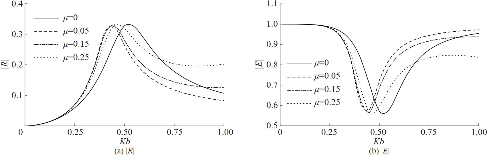Figure  19  Graph of |R| and |E| versus Kb for different values of μ with β=30° and Γ=1

Download: Full-Size Img

Graphs of the coefficient of reflection and the total energy are given in Figures 20 and 21 against the wavenumber for various α values when the porous and the impermeable barrier, respectively, are obliquely incident by waves that make an angle β=30°. They reveal that these curves attain resonant peaks when waves of certain frequency incident on the tensioned membrane barrier with a particular gap length. These peaks move towards higher values of Kb with a decrease in the tension value of the membrane. It is remarked that resonant reflections become a complete one for the impermeable membrane with a gap.

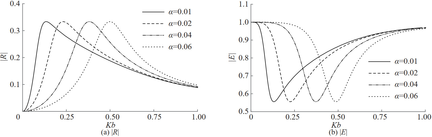Figure  20  Graph of |R| and |E| versus Kb for different values of α with μ=0.05, β=30° and Γ=1

Download: Full-Size Img

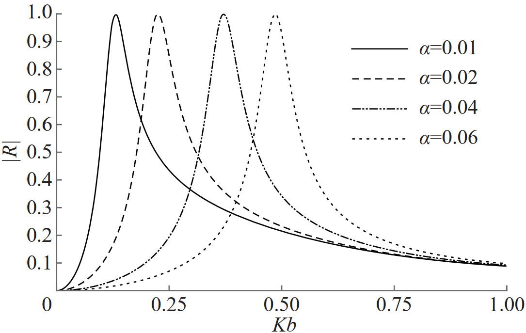Figure  21  Graph of |R| and |E| versus Kb for different values of α with μ=0.05, β=30° and Γ=0

Download: Full-Size Img

Finally, reflection and total energy curves are plotted in Figure 22 against the incident angle for various Γ values when μ=0.5, Kb=0.2 and α=0.062 46 are fixed. They reveal that the resonant peaks of these curves are attained at high incident angles as compared to the ones in Figure 17 for the case of the submerged membrane of finite length. Again, enhanced reflection is almost complete when the membrane becomes non-porous. In addition, solid porous barrier will not have any resonant reactions from the incident waves. Also, the reflection and the energy curves in Figure 23 for the solid porous barrier with a gap are comparable qualitatively with those in other barrier configurations.

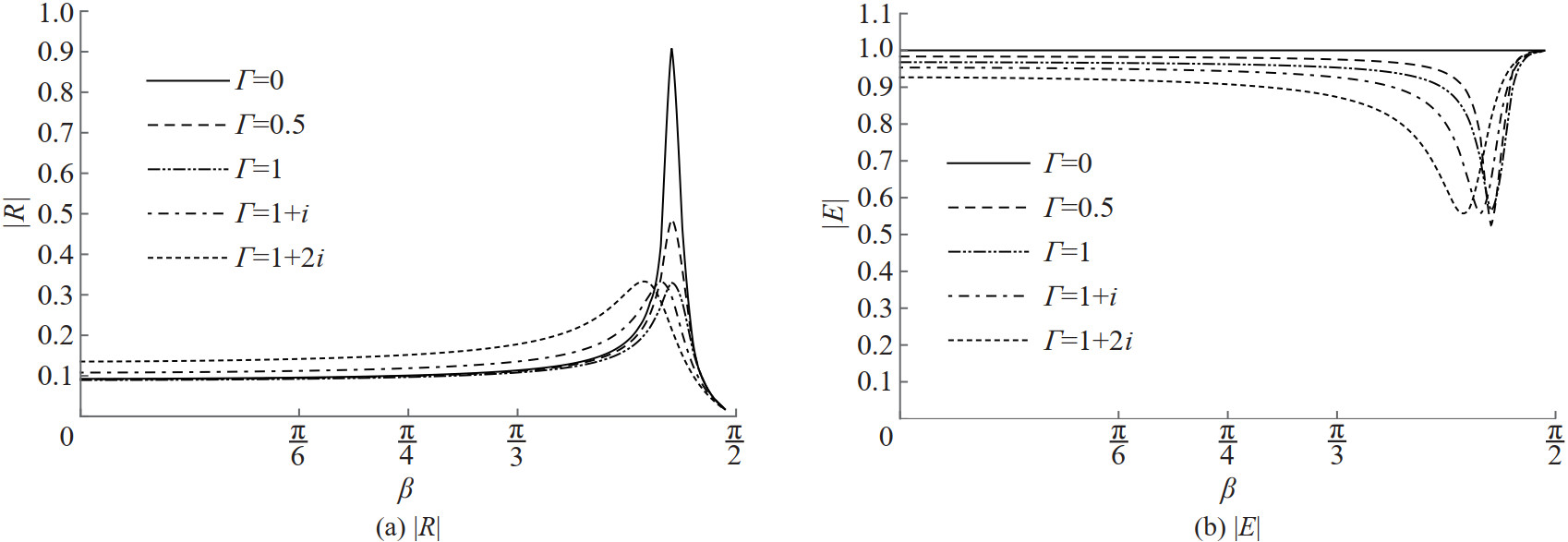Figure  22  Graph of |R| and |E| versus β for different values of Γ with μ=0.5, Kb=0.2 and α=0.062 46

Download: Full-Size Img

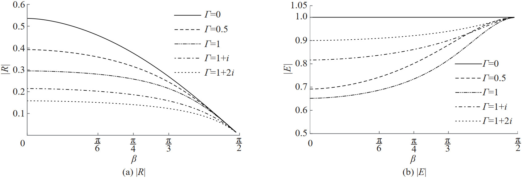Figure  23  Graph of |R| and |E| versus β for different values of Γ with μ=0.5, Kb=0.2 and α=0

Download: Full-Size Img

4   Conclusions

The present work is concerned with the scattering problem of water waves obliquely incident on four types of the vertical porous membranes such as surface piercing, submerged but finite length, submerged but infinite length and complete one with a finite gap. The original problem is decomposed into a pair of resolvable problems for the auxiliary potentials. These problems are solved by the Galerkin method with a one term or a two term approximation. Closed upper and lower bounds are obtained for the scattering quantities by choosing a suitable weight function in all the four barrier configurations. Then, the graphs of the reflection and the total energy are plotted against various parameters such as the non-dimensional wavenumber and the angle of wave incidence. Enhanced reflection and enhanced energy dissipation are found in all the four barrier configurations and they are sensitive to the incident wave angles as well as the membrane parameters. This is useful in the design of removable breakwaters such as vertical membranes by adjusting the length of the membrane suitably chosen so as to attain maximum reflection in order to mitigate harmful effects of the incident waves