1   Introduction

The analysis of multi-physics problems is important in various areas of engineering. Fluidstructure interaction (FSI) is such a multi-physics problem where the effect of the fluid on the structure could result in a significant structural deformation. This deformation affects the pressure and velocity of the fluid. Fluid-structure interaction problems are analyzed in numerical methods using two distinct approaches, a "direct" approach and a "partitioned" approach. In the first approach, the fluid and structure relations are expressed and solved simultaneously, done by Langer and Yang (2018). In the second approach, first, the fluid equations are solved for the determination of stress (traction or pressure) on solid boundaries, and then the calculated stress is used as a boundary condition for the governing equations of the structure to determine the deformation of the solid media. In fact, in the "partitioned" approach, the information is transmitted from one media to another, so that the governing equations for both media converge simultaneously (Rao and Wan 2018; Salehizadeh and Shafiei 2021).

The main drawback in solving such problems with the standard Lagrangian Finite Element Method (FEM) is that severe mesh distortions, which accompany large deformations, lead to inaccurate results. In the case of the fluidstructure interaction, the coupling of fluid and structure media is usually obtained by Arbitrary Lagrangian-Eulerian (ALE) formulations for the fluid region, while the structure is modeled with the fully Lagrangian formula, such as Aldlemy et al. (2020). Although re-meshing techniques and ALE formulations can overcome the mesh distortion issue, the remapping of state variables creates difficulties with history-dependent materials and the accuracy of results is questionable. Also, precision definition of the interface and free surfaces requires a particular remedy (Aldlemy et al. 2020).

In the last decades, the mesh-free methods have been proposed to simulate fluid-structure interaction problems, which use a fully Lagrangian formulation to describe fluid flow and structure displacement(Idelsohn et al. 2008a; 2008b; Nasar et al. 2019). These methods allow the motion of the boundary of fluid-structure interaction to be determined without any special algorithm, such as the remeshing stage (He et al. 2018). Several studies have been carried out on the development of fluid-structure interaction solvers using Lagrangian mesh-free methods. The particle modeling capability in the simulation of the breaking wave impact on a moving float is observed using Moving Particle Semi-implicit (MPS) by Koshizuka et al. (1998). Also, Lee et al. (2010) Described the MPS method for simulating the interaction of violent free-surface flow with structures. Khayyer et al. (2018b) coupled a fluid model based on MPS method with an MPS-based structure. They simulated the dam breaking with an elastic gate problem, experimented by Antoci et al. (2007) and hydro-elastic slamming of a marine panel.

On the other hand, the Smoothed Particle Hydrodynamics (SPH) method has been developed as a mesh-free Lagrangian method by Lucy (1977) and Gingold and Monaghan (1977) to solve astronomical physics problems. This method has been used in simulating various application problems such as turbulent flows (Kazemi et al. 2017; 2020), free-surface flows (Zheng et al. 2017; Salehizadeh and Shafiei 2019) and multi-material interactions (Salehizadeh and Shafiei 2021).

Due to potential advantages of SPH method, a considerable number of studies have been conducted for development of hydroelastic FSI solvers by coupling a SPH-based fluid model either with a mesh-based structure model such as SPH-FEM (Hermange et al. 2019), SPH-SFEM (Zhang et al. 2021b), SPH-ESFEM (Long et al. 2020) and SPHNMM (Xu et al. 2019). On the other hand, different FSI solvers based on pure particle methods have been developed. Zhang et al. (2021a) presented an open source SPH code named SPHinXsys to treat various FSI problems including the dam break through an elastic gate. Sun et al. (2021) developed a FSI-SPH model that is effective to solve some challenging FSI problems in three-dimensional space.

The traditional SPH solver was formulated based on a weakly compressible fluid, which relates the pressure to the variation of density through an artificial equation of state, referred as "weakly compressible" approach (WCSPH), described by Liu and Liu (2003). The standard WCSPH suffers from the computational error of density variation causes non-physical oscillations of pressure that can produce numerical instability (Lee et al. 2008). On the resolving of high-frequency pressure oscillations, extensive prevention measures have been proposed. Huang et al. (2018) employed a artificial diffusive term (δ -SPH model), proposed by (Antuono et al. 2010), to treat wave interactions with structure in field of ocean engineering. This approach requires a small time step with regard to the "sound speed", which is at least ten times higher than the maximum velocity of fluid, thus increasing computation time. To prevent such issues, the concept of "truly incompressible fluid" was achieved for SPH method. The Incompressible smoothed particle hydrodynamics method (ISPH) is a two-step method that first calculates the predicted velocity, and then the predicted values are corrected using the pressure derived from the solution of the Poisson equation to apply a divergence-free velocity field, done by Cummins and Rudman (1999).

The ISPH method can be accurate and effective in reducing the pressure fluctuations in the simulation of the fluid-solid interaction problems. Rafiee and Thiagarajan (2009) coupled the ISPH method for a fluid with an SPHbased structure. In their model, the fluid and solid pressures were determined by solving the pressure Poisson equation (PPE) with a simple scheme. They assumed that the pressure time variations are negligible between two computational time steps, which is not reasonable. Khayyer et al. (2018a) presented an enhanced ISPH-SPH coupled method for simulating fluid-structure interaction. They used a dynamic stabilizer scheme, introduced by Tsuruta et al. (2013), for fluid that involves additional calculations to determine parallel and normal vectors of predicted relative distances. Recently, their model have been demonstrated to be capable of reproducing hydroelastic FSI corresponding to composite structures (Khayyer et al. 2021).

The SPH method is applied to simulate the structural dynamics, such as in the Libersky et al. (1993) and Gray et al. (2001) studies. Antoci et al. (2007) used the WCSPH method to solve hydro-elastic problems. The original formulation of WCSPH method suffers from a series of instabilities and low accuracy issues when applied to solid mechanics (Swegle et al. 1995; Rabczuk and Belytschko 2004). The first issue SPH suffered from was the so-called "tensile instability" which leads to particle sticking and numerical fracture. To reduce the effects of tensile instabilities in solving such problems, several treatments have been proposed such as normalizing kernel functions (Johnson and Beissel 1996) and applying artificial stress (Gray et al. 2001). Nevertheless, some techniques add numerical parameters that need to be carefully selected. To eliminate instabilities related to rank deficiency in particle-based FSI modeling, Rabczuk et al. (2010) applied stress point integration (Rabczuk and Belytschko 2004) into FSI for fracturing shell structures. The stress-points implemented in mesh-free methods require a background grid for nodal integration; hence the method is not truly mesh-free. In the stability analysis of numerical mesh-free methods, Belytschko et al. (2000) found tensile instability to be caused by the use of Eulerian kernel functions. They proposed a fully Lagrangian particle method in which the initial configuration is considered as a reference, the smoothing kernel function and its derivatives are calculated based on the initial distribution of the particles, making Lagrangian kernel functions. In the present study, a totally Lagrangian formulation proposed by Lin et al. (2015) is used to the simulation of two-dimensional elastic structures. It can directly impose the interaction values such as force and velocity to the structure particles in the interaction with the fluid. The performance of the structure model is validated by simulating a cantilever beam under the concentrated force and the dynamic response of a free oscillating plate. The numerical results are compared to their analytical solution. Sun et al. (2019) introduced a coupled FSI-SPH solver by combining a multi-phase δ-SPH scheme and a Total-Lagrangian SPH (TLSPH) solver for elastic structures. In their study, the numerical results of TLSPH demonstrated sufficient accuracy and therefore, this structural solver could be further implemented in the FSI simulations. Recently, Zhan et al. (2019) and O'Connor and Rogers (2021) developed a GPU-accelerated coupled total Lagrangian and weakly compressible SPH (TL-WC SPH) approach for 3D fluid-structure interaction modeling.

The temporal pressure noise due to irregular particle distribution through clustering or stretching, leads to numerical instability. It also causes inaccurate behavior of fluid and structure in interaction with each other. A study conducted by Xu et al. (2009), enhanced particle uniformity by shifting particles slightly away from the streamlines. The hydrodynamic properties are modified after they are shifted to account for their new spatial positions by using Taylor expansion. Their method provides a stable and converged solution for fluid flow problems especially at relatively high Reynolds numbers. However, this algorithm works inaccurately in the simulation of free-surface flows due to errors associated with the truncated kernels. Lind et al. (2012) proposed a relation based on the reference concentration gradient to control normal diffusion for freesurface particles. This remedy requires the setting of the constant parameters that encounter numerical challenges in long-term simulations. To achieve an accurate and consistent implementation of particle shifting for free-surface flows, Khayyer et al. (2017) proposed a so-called Optimized Particle Shifting (OPS) scheme through a careful implementation of only tangential shifting for free-surface and free surface vicinity particles.

In this research, for the first time, a novel FSI algorithm is introduced such a way that the proposed FSI particle shifting method added to FSI coupling scheme based on ISPH approach in order that the interaction term is obtained and then imposed on the particles. This algorithm improves the interface behavior between fluid and structure. To the best of our knowledge, this is the first application of the particle shifting treatment scheme, together with the coupled algorithm into the context of simulations of FSI problems by combining an ISPH scheme and a Total-Lagrangian Particle (TLP) solver for deformable elastic structures. The developed SPH coupling method was used to simulate the interaction of fluid-elastic structures for various problems and was compared and validated with experimental results. The considered problems of fluid-structure interaction in this paper include the deflection of an elastic plate due to the hydrostatic weight of water column, done by Fourey et al. (2017), the dambreaking flow through an elastic gate, done by Antoci et al. (2007), breaking dam flow on a hypo-elastic baffle, experimented by Liao et al. (2015), the deflection of an elastic baffle due to fluid sloshing in a rolling tank, experimented by Idelsohn et al. (2008a).

2   Numerical procedure

In the SPH formulation, the particle approximation of variable A(r) is determined by a summation of particles inside the support domain of the particle located at r_a:

where V_b is the volume of particle b, h is the smoothing length which represents the discretization scale of SPH approximations and |r_ab| = |r_a − r_b| is the distance between particles a and b. In this paper, the cubic B-spline kernel is used for all cases, reviewed by Liu and Liu (2003). A smoothing length of h=1.2Δx is typically used, where Δx is the initial particle spacing. Hereafter W(|r_ab|, h)will be simply written as W_ab.

The SPH discretization of gradient, divergence and Laplacian operator for an arbitrary scalar function f or tensor function F are, respectively, calculated as:

where $ {\nabla _a}{W_{ab}} = \frac{1}{h}\frac{{\partial W}}{{\partial \left| {{\mathit{\boldsymbol{r}}_{ab}}} \right|}}{\mathit{\boldsymbol{e}}_{ab}}$ is the kernel function gradient with respect to $ {\mathit{\boldsymbol{r}}_a}{\rm{, }}\;\;{\mathit{\boldsymbol{e}}_{ab}} = \frac{{{\mathit{\boldsymbol{r}}_{ab}}}}{{\left| {{\mathit{\boldsymbol{r}}_{ab}}} \right|}}$ is the unit vector between two particles a and b; B is the corrective tensor for kernel function gradient, introduced by Bonet and Lok (1999):

and $ {\mathit{\boldsymbol{\widehat B}}_a}$ is a renormalization tensor for the second derivative given by Fatehi and Manzari (2012):

where

and $ \otimes $ defines the dyadic product of two vectors.

2.1   The projection-based incompressible SPH algorithm

In the SPH method, the Navier-Stokes equations are solved in the projection-based framework, as expressed in the Lagrangian form:

where u is the velocity field, ρ is the fluid density, p is pressure, v is kinetic viscosity, g is the gravity acceleration and v^t is the eddy viscosity due to spatial filtering. In Eq. (9), the acceleration a^{s → f} is due to the interaction force on the fluid by the structure. We used the eddy viscosity approach based on the sub-particle scale turbulence model presented by Gotoh et al. (2000):

where $ {\dot \varepsilon }_{ij}$ is the strain rate tensor; c_s is the Smagorinsky constant which is considered to be 0.1 for all simulations and Δ is the filter width, which is defined to be the SPH kernel smoothing length h. The ISPH method has been introduced by Cummins and Rudman (1999) and has been further developed by other researchers (Shao and Lo 2003; Hu and Adams 2007; Lind et al. 2012). In this approach, both the mass conversation equation and the equation of state are replaced by a Poisson equation, which is determined using the projection method. In general, to determine an intermediate velocity field, the momentum equation is solved without the effect of a pressure gradient. Then a Poisson equation for pressure is obtained by setting the divergence of intermediate velocity equal to the divergence of pressure gradient. The final velocity at the end of the time step is achieved in such a way that it results in incompressible conditions.

The ISPH solver in its original formulation suffers from the density error accumulation and errors in velocity divergence field. Several studies have been conducted to prevent such issues. Shao and Lo (2003) proposed an algorithm by imposing invariant density instead of zero velocity divergence that, despite its stability, is not accurate. Hu and Adams (2007) developed an iterative algorithm by simultaneously enforcing invariant density and zero velocity divergence that, despite its stability and accuracy, is very time-consuming. Xu et al. (2009) presented a new method to prevent the instability resulting from the intense clustering of particles. In their method, at the end of each time step, the particles are shifted away from the streamline leading to the uniform distribution of particles. Lind et al. (2012) proposed a generalized version of this scheme to allow extended applications to free-surface flows. Skillen et al. (2013) proposed a new method in the ISPH simulations for reducing the temporary disturbances caused by free surface effects. Their method provided a smoothing Poisson equation using a proposed relationship for adjacent free-surface particles. Also, the standard GPU implementation have been presented for the ISPH simulations, where the pressure Poisson equation is also solved on the GPU (Chow et al. 2018).

Here a first-order time marching scheme is applied, where both the density and mass of particles are constant; The particle positions are predicted using current velocity field:

The intermediate velocity field is calculated based on the momentum equation, regardless of pressure gradient term at the position r_a^*:

where

In which $ \bar \mu _{ab}^e = \left({{\rho _a}v_a^e + {\rho _b}v_b^e} \right)$ and $ {v^e} = v + {v^t}$. The pressure p at time n+1 can then be obtained from the pressure Poisson equation (PPE), written as:

The SPH discretized form of Eq. (14) is calculated as:

Skillen et al. (2013) proposed a suitable method for obtaining a smoothing pressure field at the free-surface. By identifying the particles on the free-surface and adjacent to the free-surface, a variable correction coefficient is used which leads to effect of free-surface gradually. The freesurface particles are detected by calculating the divergence of the position vector of particles. By detecting the freesurface particles, these particles are given a zero pressure over a time step (Dirichlet condition in the Poisson equation of pressure). After the discretization of the Eq. (15), the Poisson equation of pressure is rewritten in the following form:

where A_ab are the Poisson's coefficients of pressure and the summation is applied to all particles located in the support domain of the particle a. It is noted that the calculation of new pressures (pⁿ⁺¹) requires a limited number of iterations to reach the smoothing converged pressures. The coefficient appearing in Eq. (16) is proposed by Skillen et al. (2013) for the implementation of the effect of free surface conditions, which follows:

Then, by calculating the pressure of particles, the velocity at the end of the time step is determined from the intermediate velocity and the negative version of pressure gradient:

In the end, the position of the particles is updated as follows:

In order to stabilize the simulation and form a uniform distribution of particles, after the particle positions are advanced in time by Eq.(19), following Xu et al. (2009), the particles are shifted slightly, then the hydrodynamic variables are corrected by the Taylor series approximation:

where A is a general variable; a and α′ are the particle's old position and new position respectively; δr_aa′ is the displacement vector between the particle's new position and its old position. By modifying the particle shifting magnitude, ζ, in relation to the particle convection distance and the particle size, the position shift reads:

where C is a constant in the range of 0.01 −0.1; ζ is the shifting magnitude which is equal to the maximum particle convection distance |u|_maxΔt, with |u|_max the maximum particle velocity, and Δt the time step; R_a is solved by following equation:

where N_a is the number of neighboring particles around particle a, is the distance between particle a and particle b, and n_ab is the unit displacement vector between particle a and b; r_a is the average particle spacing in the neighborhood of a, and reads:

Lind et al. (2012) observed that due to the motion of free-surface particles, the distance of particle displacement would be much greater than the smoothing length which results in an irrational error; therefore, an upper limit for the particle shifting distance was defined as 0.2 h. The incomplete kernel support and increased kernel interpolation error in free-surface regions, lead to error in determination of the displacement vector of particles.

According to Khayyer et al. (2017), in the area near the free surface, the shifting distance of the fluid particles was forced to be equal to zero in the normal direction of the free surface. To achieve a reliable physical particle shifting for free-surface and nearby particles, the particle shifting displacement vector for these particles is modified by Khayyer et al. (2017) as follows:

where Δr_a is obtained by Eq.(21). For the free-surface particles, the normal vector is determined by:

where

Figure 1 shows the particle shifting process for a free surface particle. The particles as depicted in Figure 2, are determined in the simulation as internal particles, particles adjacent to the free surface, free-surface particles and splash particles based on the divergence of the position vector of particles. At first, the free-surface particles are determined based on the divergence of position vector ∇·r < x and the normal vector is obtained for them. Then the adjacent particles to the free surface are determined based on the establishment of two criteria of the divergence of position vector x < ∇·r and the spatial distance |r_a′b| < h (a′ nearest neighbor particle in the free surface to the particle b) and the normal vector of the nearest neighbor particle located on the free surface is assigned to these particles. Splash particles have the divergence of position vector ∇·r < x which do not have any neighboring particles in their support domain. By detecting free-surface and nearby particles and also splash particles, the internal particles are distinguished. It should be noted that for splash particles, the correction coefficient is zero. In the present study, the value of x was chosen to be 1.4.

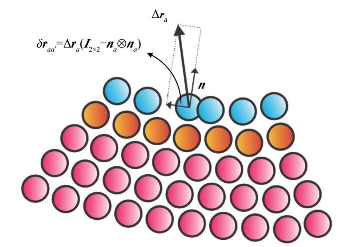Figure  1  The particle shifting process for a free-surface particle (Khayyer et al. 2017)

Download: Full-Size Img

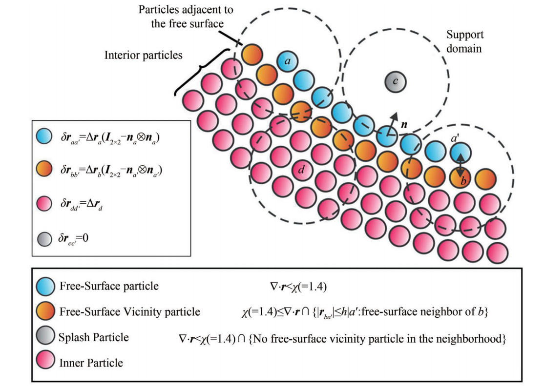Figure  2  Particle status identification to calculate the vector of particle displacement

Download: Full-Size Img

Within discontinuous regions on the surface of the structure, the large displacements lead to instability, which result in forming jamming clumps due to disrupt of the fluid particles adjacent to the surface of the structure. To solve this problem, a novel method is proposed to shift the fluid particles adjacent to the surface of the structure. An intermediate boundary layer is characterized in the fluid domain on surface of the structure as shown in Figure 3.

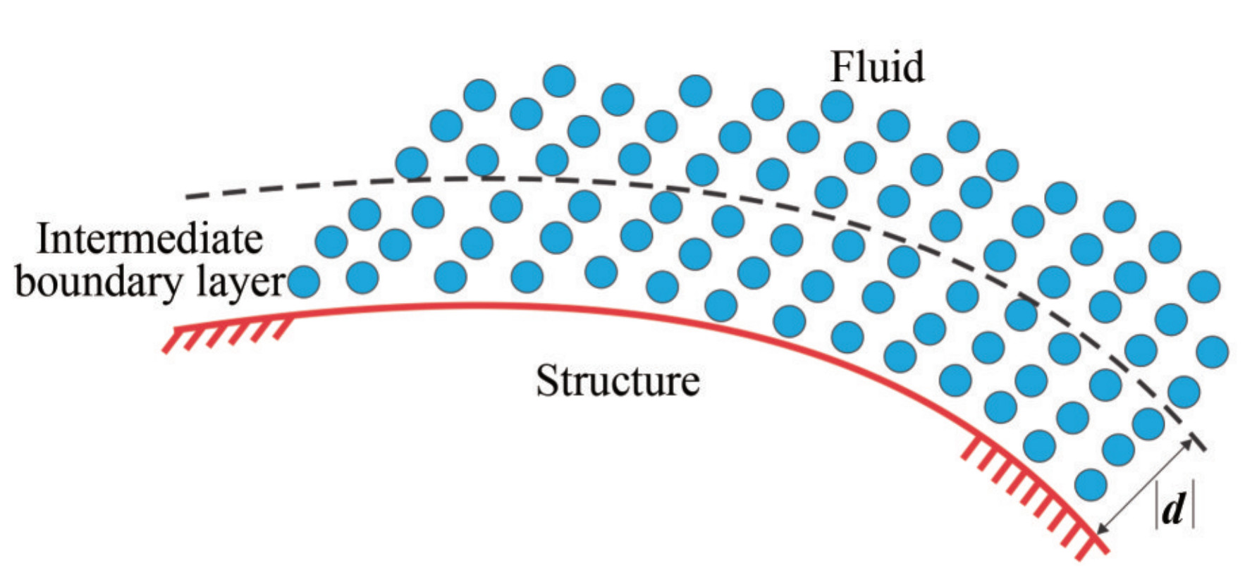Figure  3  Definition of intermediate boundary layer in fluid domain

Download: Full-Size Img

When the fluid particles are located in this intermediate boundary layer, these particles are displaced based on a predefined nonlinear function. This method results in a preserved solution with smoothing the velocity field. Relocation of fluid particles located in the intermediate boundary layer is executed using an exponential function.

where δr_aa′·n_a is prescribed displacement vector by Eq. (21) in local normal direction n of the boundary surface and d is a flow dependent vector in local normal direction n. Considering a large depth for the intermediate boundary layer, |d|, enhance the stability of the solution with increasing the number of particles within the layer that need to be relocated. Applying this relocation is determined with defining limits for |d|. If the value of δr_aa′|_n is assumed to be equal to |u|_maxΔt and δr_aa′|_new is limited to the shifting distance proposed in Eq.(21) in local normal direction n, Eq. (27) becomes:

By applying second order Taylor series to scalar form of Eq. (28), it becomes:

where C is a constant parameter in the range of 0.01‒0.1, limits for |d| can be determined:

Finally, the hydrodynamic variables of modified at the new position as follows:

2.2   Total lagrangian formulation for elastic structures

The Total Lagrangian SPH (TLSPH) method is applied by Lin et al. (2015) to model the elastic structures; in this formulation, the density is considered constant and to solve the momentum equation in the reference framework, the first Piola-Kirchhoff stress tensor P^s replaces the Cauchy stress tensor σ. Therefore, Eq.(9) is given in the following form:

In the above equation, α^{f → s} is the acceleration due to the interaction force on the structure from the fluid side. The relation between P^s and σ is as follows:

It is necessary to obtain first-order consistency to avoid numerical errors caused by the truncated kernel function on the structure. For this purpose, the shape tensor is determined by Rabczuk et al. (2004) to reproduce the SPH kernel gradients correctly, as follows:

where ∇₀W_ab is the gradient of kernel function corresponds to particles a and b in their initial configuration as the subscript 0 has indicated, and X is a coordinate in the reference configuration. N_b represents the number of structure particles in the support domain of particle a. The deformation gradient tensor F is approximated as follows:

where x is coordinate vectors in the current configuration. The Cauchy stress σ_ij (i and j represent coordinate vectors) based on Eulerian strain ε_ij is determined in two dimensions by Hooke's law for an isotropic elastic material:

For the plane-strain problem and,

For the plane-stress problem. Accordingly, v_s is Poisson's ratio and, E_s is Young's moduli. The Eulerian strains are defined using the deformation gradient tensor:

Regarding non-linear geometric behavior, the Green-Lagrange strain tensor is used, as follows:

In the above relation, the displacement gradient tensor is based on the displacement vector:

The TLSPH scheme suffers from rank-deficiency of zero energy modes due to its particle arrangement nature. Therefore, the discrete form of Eq. (33) is written in the initial configuration using the first Piola-Kirchhoff stress tensor and the interaction acceleration term.

In the present study, the 4^th-order Runge-Kutta scheme as a multi-stage method is used to integrate the momentum equation (Eq. (42)) in time. This time integration scheme is fully explicit and is expressed as:

where k_um and k_rm are solved simultaneously for each stage:

where Δt is time step and a=du/dt.

2.3   The fluid-structure interaction treatment for ISPH-TLSPH model

Although the SPH method is used to solve the governing equations for both fluid and structure media, two numerical separated approaches for these media are considered. Therefore, they must be coupled together in a physically manner and applicable mathematics. In the following, the adopted algorithm for coupling is expressed and can be seen in Figure 4.

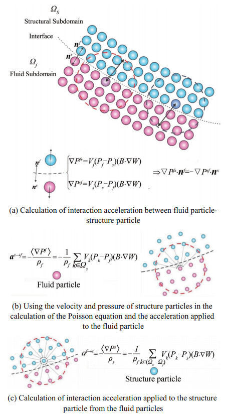Figure  4  Schematic View of the coupling model between fluid and structure

Download: Full-Size Img

Throughout the interface between fluid-structure, the normal components of the velocity vector must be continuous. For this purpose, the use of the velocity field of the structure provides a suitable boundary condition for the fluid flow. In other words, the structure particles are used as moving boundaries for fluid governing equations to complete the support domain of fluid particles.

Essentially, the normal component of Cauchy stresses in fluid and structure are continuous on the boundary of fluidstructure interaction. In assuring the normal stress continuity at the fluid-tructure interface, The pressure (an isotropic section of Cauchy stress) is considered continuous during the interaction between fluid and structure. Using the projection-based particle method, the ISPH algorithm is applied to all particles adjoining each other, regardless of their nature (belonging to the structure or fluid media). In other words, the position and velocity of structure particles as a boundary condition are used to calculate the fluid pressure field using the pressure Poisson equation (Figure 4b). The present algorithm accompanied by the proposed FSI particle shifting scheme ensures that the fluid velocity field remains free-divergence. When the fluid pressure field is calculated, the interaction term in the equation of fluid and structure momentum is determined based on the pressure gradient between the fluid and structure particles. Hence, the components of the interaction force, perpendicular to the interface of the fluid and structure, are equal in the opposite direction. According to this:

Regarding Neumann boundary condition for the pressure field across the interface of fluid-structure interaction and considering a no-slip boundary condition at the fluidstructure interface, the Eq. (46) shows the relation of normal stress continuity at the interaction boundary. By using optimized particle shifting method, the fluid particles are then shifted slightly, also, the pressure field of all particles regardless of their nature are corrected by the Taylor series approximation,

The modified pressure field of particles is used to calculate pressure gradient at a typical structure particle and then imposed on the structure particle as interaction term α^{f → s}. This proposed coupling scheme works in a robust and efficient manner so that, no internal iteration for a converged particle position is needed. The interaction term obtained on the basis of the pressure gradient for a structure particle is as follows:

where k denotes all the particles of fluid and structure in the support domain of structure particle (Figure 4(c)).

The exchange of kinematic information throughout the interaction thus leads to a coupled process for a problem with material discontinuity. The pseudo-code of the present solution algorithm is shown in Algorithm1 in the Appendix.

2.4   Time-stepping condition

In SPH method, the time step is generally determined in the Courant-Friedrich-Levy conditions:

Where Cr is Courant number and U is the characteristic velocity of the model. The SPH-based structure model and the fluid model utilize different characteristic velocities in their formulation. The sound speed is used in the structure model, while for fluid, the maximum velocity of the fluid is used in each time-step. Consequently, the time steps allowed for a structure should be quite smaller than the fluid. Therefore, significant improvements are achieved using separate and different time steps for both media. In this study, the time step of the structure Δt_s was set to 0.01 Δt_f. Therefore, the fluid governing equations are updated for every 100 steps of the structure. Here, the Courant number is taken as Cr=0.1 for all cases.

The proposed scheme is programmed in Fortran and an Intel^® Core^TM i7-4770 CPU is used to run the computations.

3   Validations and comparisons

3.1   Benchmark tests for the structural analysis

To validate the structural analysis method, static and dynamic simulations were performed on an elastic structure. In a static simulation, a concentrated load is applied to clamped beam at its end. The geometric dimensions of the clamped beam are shown in Figure 5, which L=100 mm is the length of the beam, b=1 mm the width and T=10 mm thickness of the beam. The load is gradually increased ranging from 0 to 1750 N within t=1.5 ms; then the load remains constant until the simulation ends at t=3 ms. Young's moduli and Poisson's ratio for the beam were considered E=210 GPa and v=0.3 respectively.

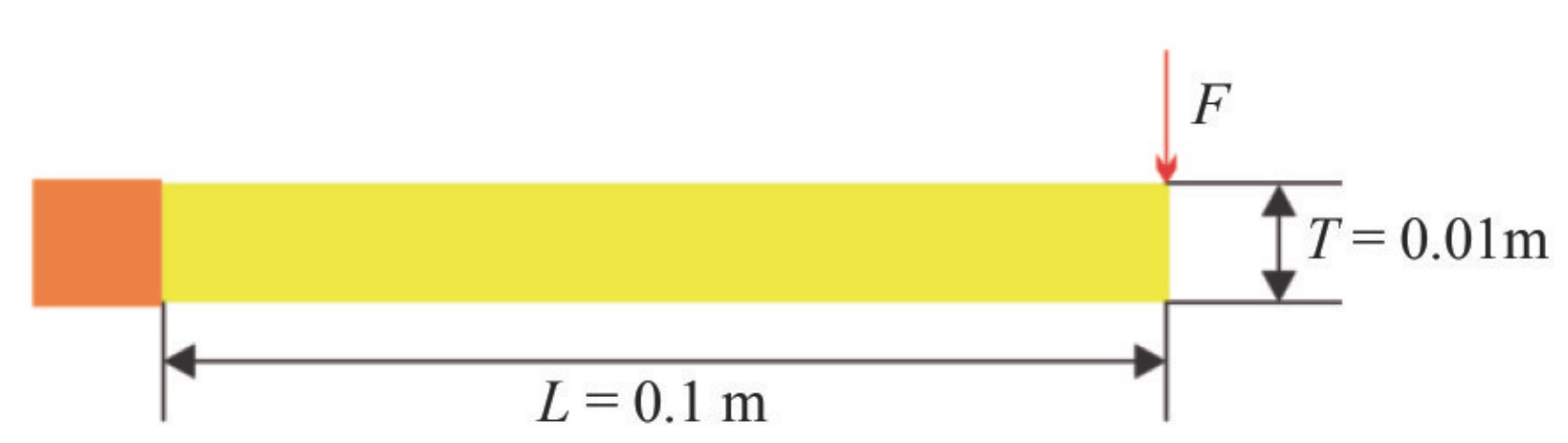Figure  5  The sketch of static problem of a clamped beam under concentrated load

Download: Full-Size Img

The maximum displacement of the beam under the concentrated load at its end is obtained by:

A sensitivity analysis of the particle discretization is carried out. The Different particle resolutions have been used, starting from N_y=5 particles through the thickness until N_y= 17 particles. For every case, the solution Δ_TLSPH/Δ is calculated and evolved vs number of particles as depicted in Figure 6. As one can observe, the predicted TLSPH enddeflection converges to the analytical solution as the number of particles is over ten, the error between the end deflection obtained using the TLSPH model and the analytical value is less than 1.04 percent, which is acceptable.

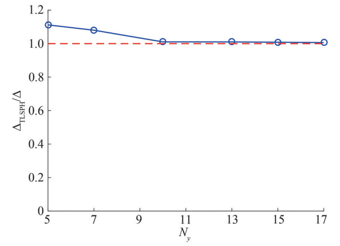Figure  6  The ratio of predicted TLSPH end-deflection to the analytical solution vs the number of particles through the thickness

Download: Full-Size Img

Table 1 presents the Root Mean Square Error (RMSE) of the results obtained from the simulations by TLSPH model presented in Figure 6.

Figure 7 shows the vertical displacement of the beam. The presented result has an acceptable correspondence with the analytical solution.

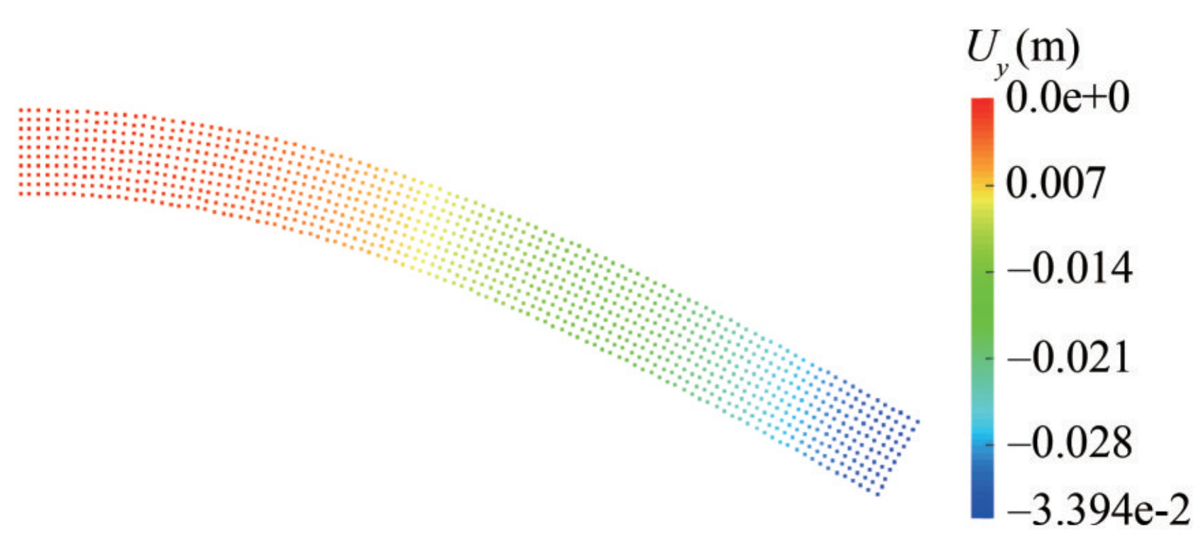Figure  7  The deformed configuration of the clamped beam and the vertical displacement distribution of the beam

Download: Full-Size Img

The present structure model was also used to simulate the free oscillation of an elastic plate of length L=0.2 m and thickness T=0.02 m with a clamped edge and free edge (Figure 8). The initial vertical velocity distribution for the elastic plate is considered as follows (Gray et al. 2001):

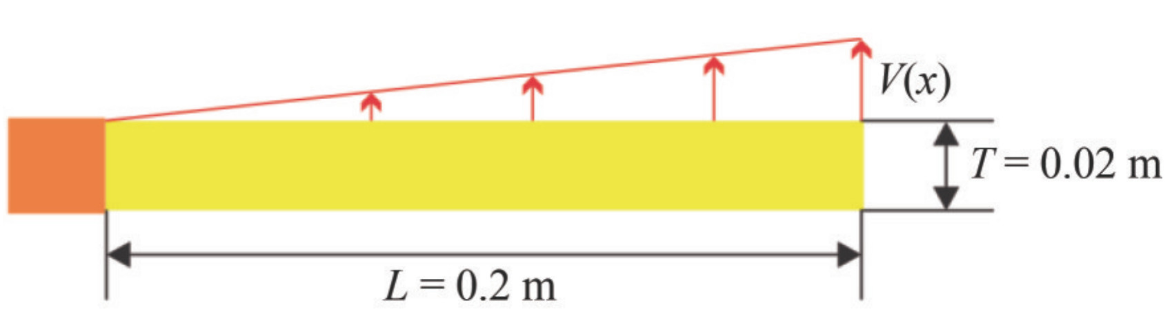Figure  8  Schematic sketch of the dynamic problem of a free oscillating plate

Download: Full-Size Img

where

where kL=1.875. V_0L=0.01 is the initial velocity at the free end and $ {c_0} = \sqrt {K/\rho } $ is the sound speed, which K is the bulk modulus of elastic plate. For comparison with the results of Antoci et al. (2007), the properties of the elastic plate were considered to be ρ=1 000 kg/m³, K=3.25 MPa and v=0.397 5. For resolution test, the particle spacings of Δx= 0.002 m, 0.001 m and 0.000 5 m are chosen which correspond to 10, 20 and 40 particles in vertical direction. The simulation results are compared with analytical solution in Figure 9. The plate tip's vertical displacement in Figure 9 shows that the present simulation is well-resolved for T/Δx =20.

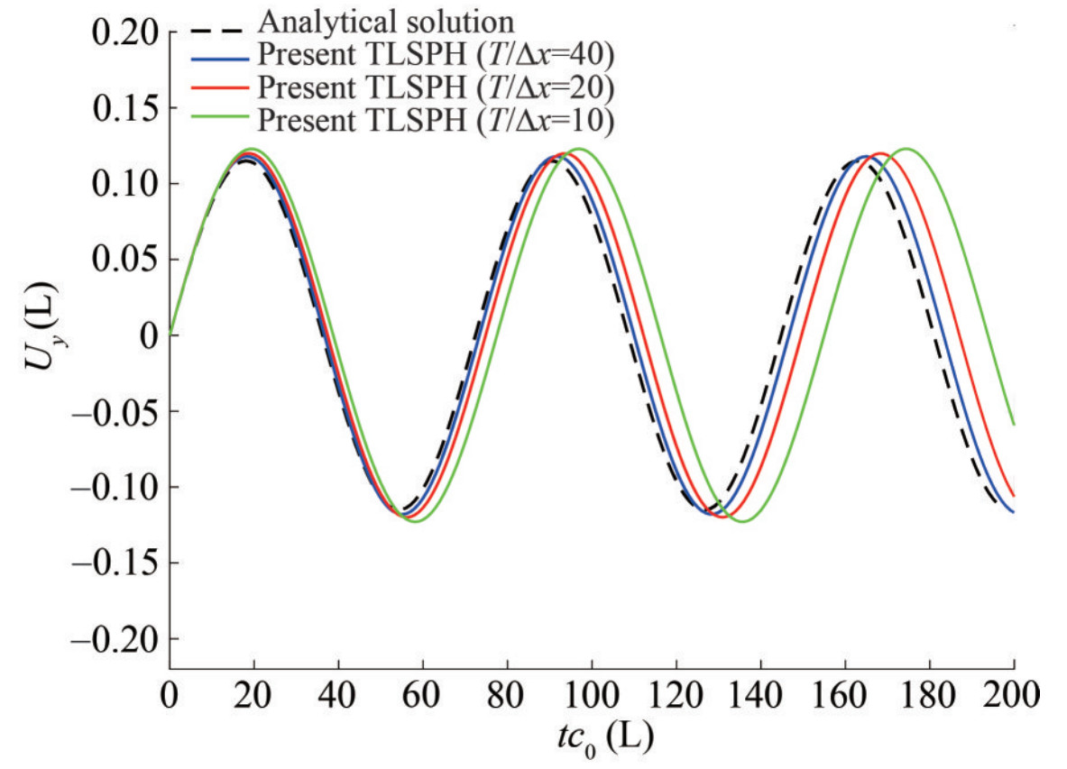Figure  9  Time histories of oscillations of the free end of the elastic plate reproduced by TLSPH with a set of different particle spacing with corresponding analytical solution

Download: Full-Size Img

Table 2 provides RMSE and Normalized Root Mean Square Error (NRMSE) corresponding to the results in Figure 9, quantitatively verifying the convergence property of the TLSPH model.

In Table 3, the simulation results are compared with analytical solution and numerical results by other researchers who had performed this test using other approaches.

Figure 10 shows the deformed configuration of the elastic plate at the maximum vertical displacement of the plate at the instant t=0.65 s (Figure 10(a)).

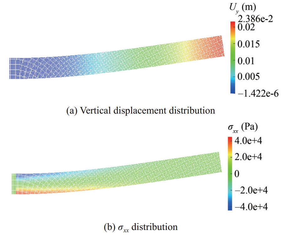Figure  10  Dynamic response of elastic plate under free oscillation

Download: Full-Size Img

In order to investigate the energy conservation property of 2D TLSPH model, time histories of kinetic, elastic strain, total energies until t=0.7 s are presented in Figure 11. The presented time histories correspond to particle spacing of Δx=5.0e-4 m. From the presented figure, kinetic and elastic strain energies consistently vary in time with a phase difference of half of the period of plate's oscillatory motion

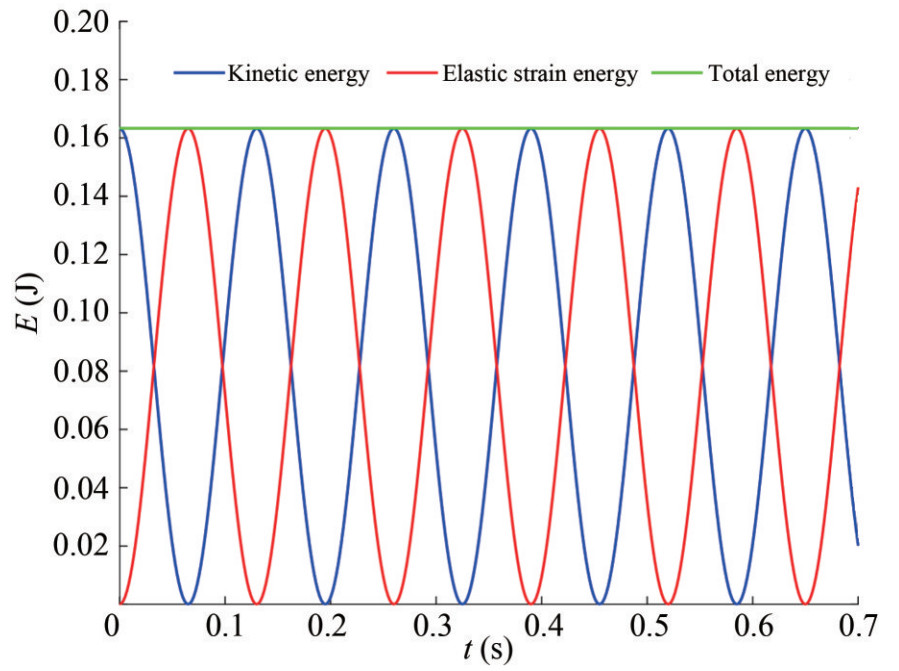Figure  11  Time histories of kinetic, elastic strain, total energies by 2D TLSPH — dynamic response of a free oscillating elastic plate

Download: Full-Size Img

3.2   Benchmark tests for the fluid-structure interaction

The proposed algorithm for analyzing fluidstructure interaction problems is evaluated through several examples of applied problems.

3.2.1   Hydrostatic column of water on aluminum elastic plate

Figure 12 shows the initial configuration of the problem. An elastic aluminum plate with a width L=1m and a thickness T=0.05 m clamped on both sides and the column of water to the depth of H=2 m with a similar width at the top of the plate. Water pressure variation is due to the effect of gravity. For the fluid, density and dynamic viscosity were ρ_w=1000 kg/m³ and μ_ω=1.0×10^-3 Pas respectively, and the physical parameters of the aluminum plate were considered ρ_s=2700 kg/m³, E=67.5 GPa and v=0.34.

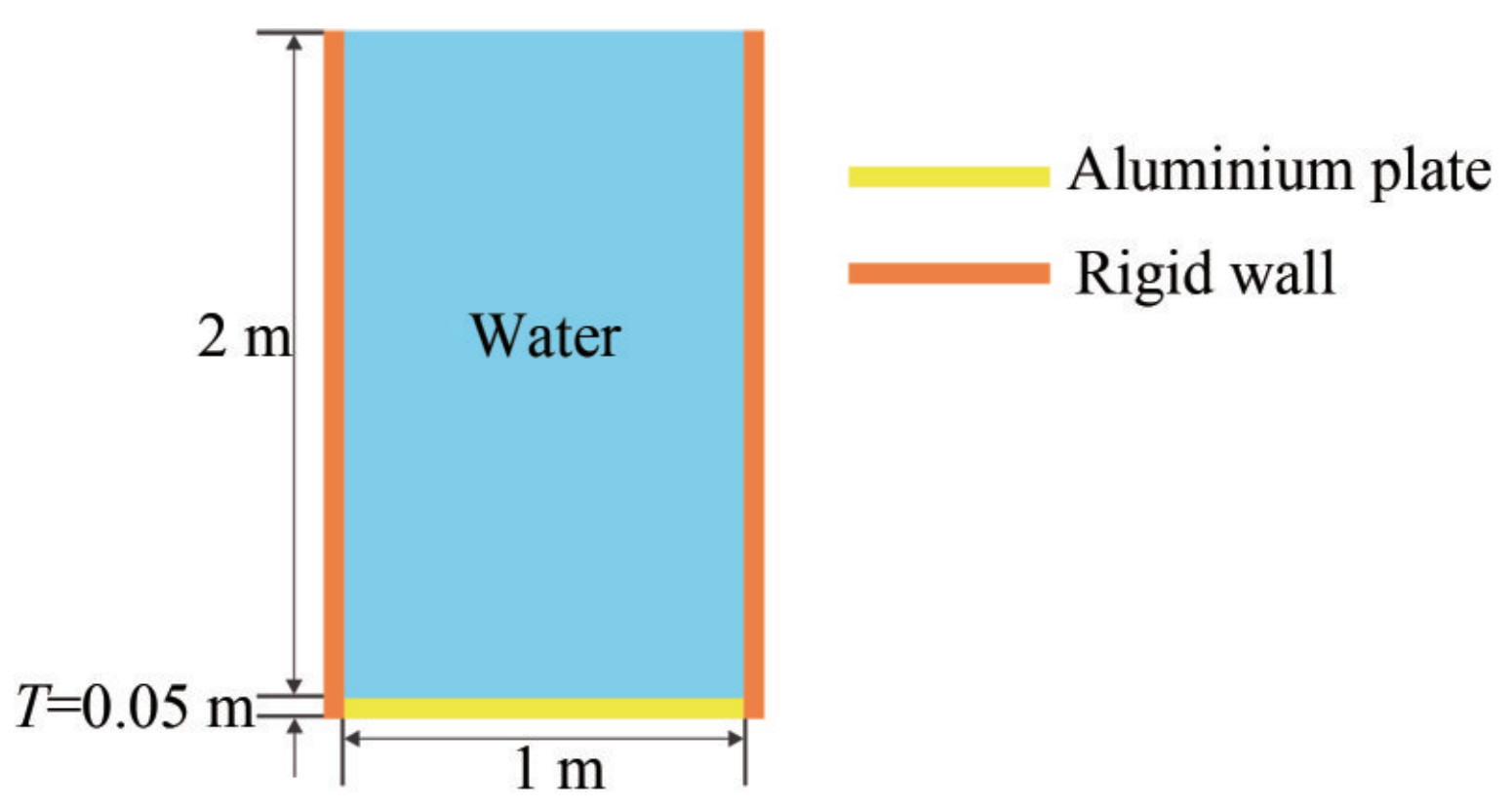Figure  12  Schematic sketch of hydrostatic water column on an aluminum elastic plate

Download: Full-Size Img

First, the aluminum plate bends due to the weight of the water column and the weight of the plate. Then, with the energy transfer between the potential energy and the kinetic energy, the elastic plate vibrates around its equilibrium state. The average mean descent of the elastic plate with the assumption of no damping in the structure and no viscosity in fluid, is calculated based on static analysis:

Figure 13 presents a set of time histories of plate's midspan deflection U_y corresponding to three different spatial resolutions (initial particle spacing) by refining the resolution from T/Δx=8 to T/Δx=12. The accuracy of deflection time history increases and eventually, for T/Δx=12 is quite well consistent with theoretical static displacement. In the beginning, the aluminum plate falls under sudden load caused by the weight of the water column. In the following, the plate vibrates in response to this extensive load. Progressively, the plate damped and remains close to its static point. The acceptable stability was obtained by using the fluid-structure interaction algorithm based on the SPH method and a noise-free pressure field was provided.

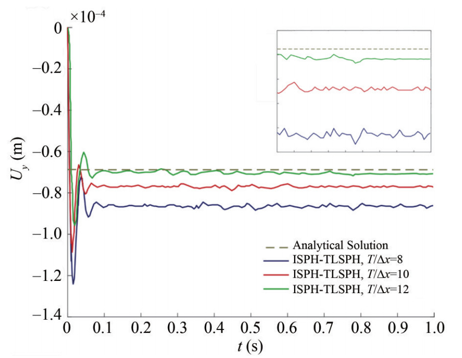Figure  13  The time histories of deflection at the midspan of an elastic plate under hydrostatic water column simulated by ISPHTLSPH FSI solver with respect to the analytical solution

Download: Full-Size Img

Table 4 presents the RMSE corresponding to numerical results shown in Figure 13.

Figure 14 shows the vertical displacement of the center of the elastic plate Uy during the time for T/Δx=12 as compared to the Fourey et al. (2017) results.

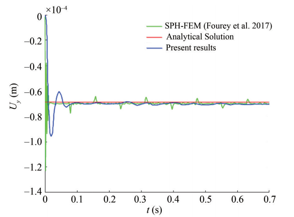Figure  14  The time histories of deflection at the mid-span of an elastic plate under hydrostatic water column

Download: Full-Size Img

Figure 15 shows the fluid pressure field and stress distribution of the structure reproduced by ISPH-TLSPH coupled method at t=0.3 s. The computational conditions for the corresponding simulation are T/Δx=12 and Δt_max^f = 8.0e-6 s.

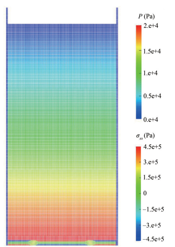Figure  15  The fluid pressure field and stress distribution of the structure at t=0.3 s

Download: Full-Size Img

In addition, Table 5 shows the required CPU time for ISPH fluid model and SPH structure model for one second of simulation of the hydrostatic water column on elastic plate for the resolution of T/Δx=12.

3.2.2   Dam breaking through an elastic gate

The problem of water dam-breaking through an elastic gate was considered in comparison with the experimental results presented in Antoci et al. (2007) and the numerical results (Antoci et al. 2007; Rafiee and Thiagarajan 2009; Khayyer et al. 2018a; Fourey et al. 2017). The initial configuration of the problem is shown in Figure 16. The water is located inside a reservoir that can flow by pushing a deformable gate that is clamped from above to a rigid wall. The elastic rubber gate is of thickness T=5 mm with density ρ_gate=1 100 kg/m³, Young modulus E=12 MPa, and Poisson ratio v=0.4.

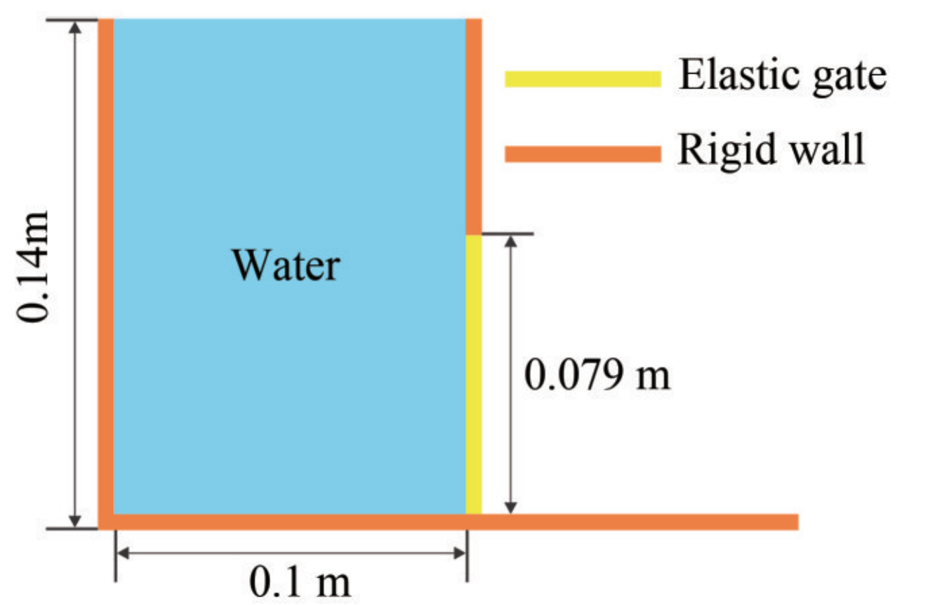Figure  16  Schematic sketch of the test case: breaking-dam flow through an elastic gate

Download: Full-Size Img

The comparison between experimental results and numerical simulation is shown in Figure 17 for every 0.04 seconds. The hydrostatic pressure of water causes the gate to gradually open, resulting in water flowing. By increasing the gate opening, the amount of water leakage is intensified. With the passing of time at the instant t≈0.14 s, the pressure applied on the back of the gate decreases due to the lowering of the water surface. Therefore, the gate slowly returns to its initial position.

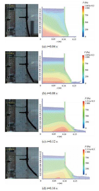Figure  17  Qualitative comparison between simulation snapshots and experimental photographs, obtained by Antoci et al. (2007) for every 0.04 second in breaking-dam flow through an elastic gate

Download: Full-Size Img

The distribution of stresses σ_xx and σ_yy for the elastic structure at its maximum vertical displacement at the instant t≈0.14 s is shown in Figure 18.

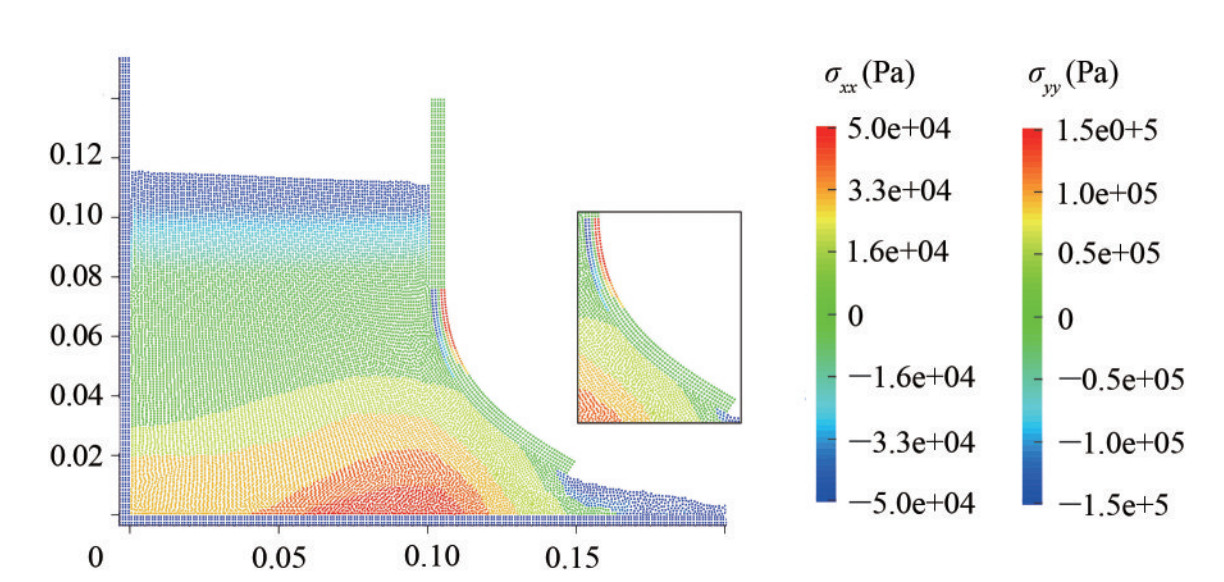Figure  18  The distribution of stresses σ_xx and σ_yy for the elastic structure reproduced by ISPH-TLSPH coupled method at its maximum displacement

Download: Full-Size Img

Figures 19(a) and 19(b) show the horizontal and vertical displacement of the free end of the gate in time to compare with the results of Antoci et al. (2007) (experimental, WCSPH), Rafiee and Thiagarajan (2009) (ISPHWCSPH), Khayyer et al. (2018a) (ISPH-SPH) and Fourey et al. (2017) (SPH-FEM). As can be seen, at the moment t≈ 0.14 s, the elastic plate reaches its maximum vertical displacement. The results show that the proposed coupled algorithm for structure-fluid interaction analysis provides acceptable accuracy for determining the displacement of the elastic gate. It should be noted that the difference between the results of the present study and the experiments of Antoci et al. (2007) is due to the nonlinear behavior of the rubber gate in the experiment. Comparison of the results of the present study with other studies shows that the different treatment of incompressible constraint of fluid in weakly compressible approach and truly incompressible approach (based on the SPH method) and different structural models lead to a difference in the determination of the amount of displacement of the gate.

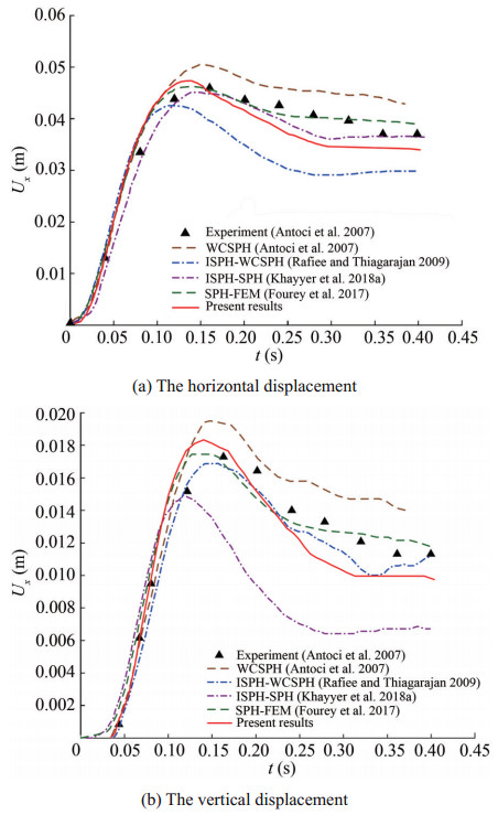Figure  19  Time histories of the displacement of the gate's free end; present results by ISPH-TLSPH model vs. experimental results (Antoci et al. 2007) and numerical results (Antoci et al. 2007; Rafiee and Thiagarajan 2009; Khayyer et al. 2018a; Fourey et al. 2017)

Download: Full-Size Img

The energy conservation property of ISPH-TLSPH FSI solver is investigated in the benchmark test of dam breaking through an elastic gate by considering the energy components corresponding to fluid and structure. The effect of elastic energy of fluid due to compressibility is neglected by considering an incompressible fluid within the context of ISPH. The time evolution of the mechanical energy of the coupled system in each sub-domain is presented in Figures 20(a)‒20(e) as well as the energy accumulated at the fluid-solid interface in Figure 20(f).

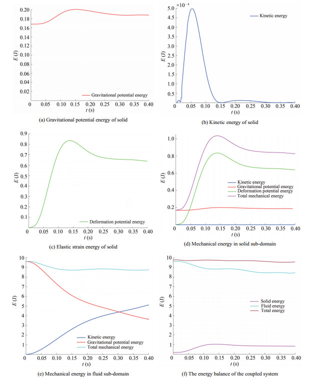Figure  20  Time histories of Mechanical energy in structure and fluid sub-domain and energy balance for the whole coupled system

Download: Full-Size Img

Figures 20(a), 20(b) and 20(c) show the time variations of gravitational potential energy of structure, the kinetic energy of structure and elastic strain energy of the structure, respectively. Figure 20(d) illustrates the time evolution of the mechanical energy of the coupled system in structure sub-domain. Figure 20(e) shows the time evolution of the mechanical energy of the coupled system in fluid sub-domain. From Figure 20(e), this drop of energy is mainly linked with the drop in gravitational potential energy of fluid. Figure 20(f) presents the time histories of total energy of the FSI system. A slight decreasing of the total system energy is observed that can be interpreted as a slight numerical dissipation. Indeed, within the context of ISPH, the fluid is considered to be incompressible and thus, the elastic energy of fluid due to compressibility is ignored. For the considered benchmark test, the proposed ISPH-SPH FSI solver is shown to possess acceptable energy conservation properties.

3.2.3   Breaking dam on a hypo-elastic baffle

In order to investigate the interaction of fluid-structure with free-surface and the proposed algorithm for the particle shifting scheme concerning the free surface, numerical simulations of the collision of a water column with an elastic baffle are discussed. The computational condition of the benchmark test corresponds to the experiment by Liao et al. (2015). The schematic sketch of the problem is illustrated in Figure 21. The elastic plate is of T=0.004 m thick with Young's modulus and density of E=3.5 MPa and ρ=1 161.54 kg/m³, respectively.

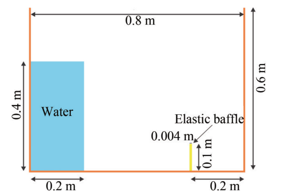Figure  21  Schematic sketch of the test case: breaking dam on a hypo-elastic baffle based on Liao et al. (2015) experiment

Download: Full-Size Img

Figure 22 presents a set of snapshots corresponding to the simulation of water dam-breaking on an elastic baffle versus the experimental results at 0.25 s < t < 0.75 s. By comparing the present numerical results with experimental data, done by Liao et al. (2015), It is observed that the developed coupled algorithm based on SPH method determines the main characteristics of the phenomenon of breaking dam on an elastic baffle. As shown in Figure 22, in the early stages of the impact of the fluid on the elastic structure, an acceptable accuracy is obtained with respect to the baffle movement. With time passing, track of the blade tip shows oscillation in the experiment; however, numerical results do not show clearly these vibrations.

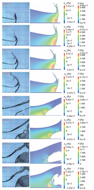Figure  22  Qualitative comparison between simulation snapshots and experimental photographs, obtained by Liao et al. (2015) in breaking-dam flow on an elastic baffle: fluid pressure field and stress component σ_yy in structure

Download: Full-Size Img

Hence, the horizontal displacement of the blade tip continues to the right and then moves to its stable point by fluid accumulation in two sides of the obstacle. The application of the proposed particle regularization scheme is effective for elimination of pressure oscillations, in particular for interaction regions. The configurations of freesurface fluid flow and deformed baffle are qualitatively well reproduced compared with those of experimental results by Liao et al. (2015). Despite the local fluctuations in the pressure field, the reproduced pressure/stress fields obtained from the simulation are consistent with the numerical results of Khayyer et al. (2019). Figure 23 shows the time histories of the displacements of the baffle's free end U_x reproduced by proposed SPH-based FSI solver along with corresponding experimental data (Liao et al. 2015) and the numerical results by FDM-FEM (Liao et al. 2015), multi-resolution MPS (Khayyer et al. 2019), single-phase δ-WCSPH-TLSPH scheme (Sun et al. 2019) and multi-phase δ-WCSPH-TLSPH scheme (Sun et al. 2019).

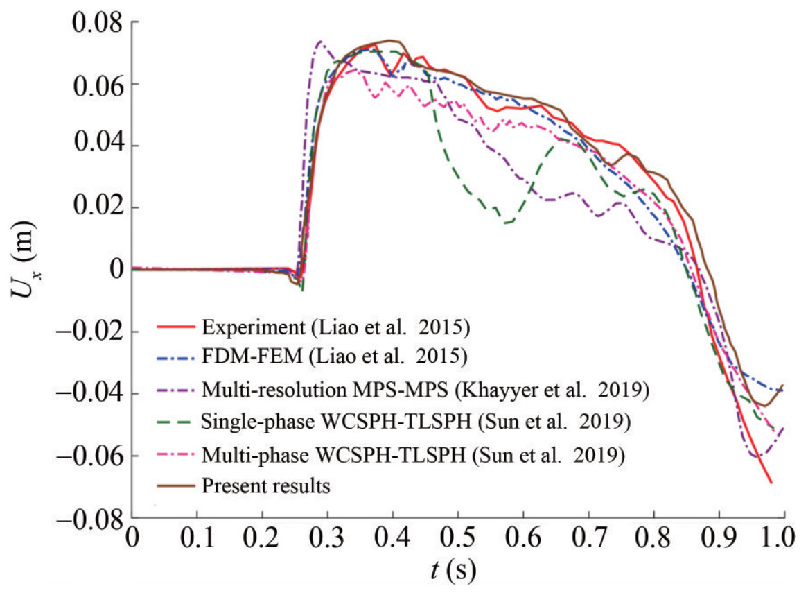Figure  23  Time histories of the horizontal displacement of the free end of baffle; present results by ISPH-TLSPH model vs. experimental results (Liao et al. 2015) and numerical results (Liao et al. 2015; Khayyer et al. 2019; Sun et al. 2019) - Breaking dam on an elastic baffle

Download: Full-Size Img

It can be seen that the proposed SPH-based coupled method has provided an almost acceptable level of accuracy with the experimental result. To study this test case more precisely, the proposed algorithm is used for simulation this problem with different geometry followed by other numerical studies. This configuration has been studied by other researchers using finite element method (FEM), simulated by Walhorn et al. (2005), particle finite element method (PFEM), done by Idelsohn et al. (2008b) and ISPH-WCSPH coupled method, simulated by Rafiee and Thiagarajan (2009). Although there are no experimental results for this configuration, however, the free surface profile and the elastic baffle deformation correspond to the physics of the problem. The initial configuration of the problem is presented in Figure 24. A column of water placed in hydrostatic equilibrium in a reservoir, and an elastic baffle with density ρ_b=2500 kg/m³, Young modulus E=1 MPa, and Poisson ratio v=0 in the middle of the reservoir is clamped from below. The geometry of the elastic baffle is width B=1.2 cm and height H=20/3B. The sound speed of the fluid c_w=50 m/s and the initial distance between the particles Δx=2.4 mm were considered.

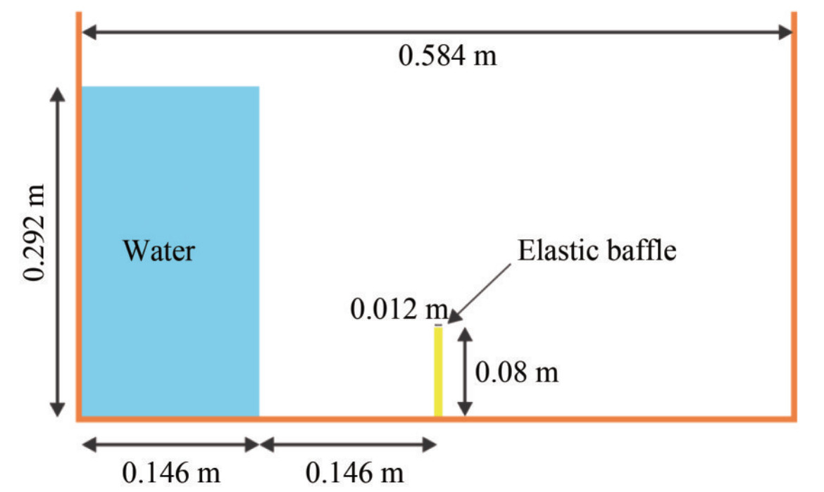Figure  24  Schematic sketch of breaking dam on an hypo-elastic baffle based on numerical studies (Idel-sohn et al. 2008b; Rafiee and Thiagarajan 2009; Walhorn et al. 2005)

Download: Full-Size Img

Figure 25 shows the fluid pressure field and the stress component σ_yy of the elastic structure. When the fluid encounters a baffle, because of the impact of the fluid on the lower part of the obstacle, firstly, its free end is diverted to the left. And by increasing the amount of water behind the obstacle, the baffle moves to the right. The maximum deviation of the obstacle to the right occurs when water jets pass through it, and the left side of the baffle is completely under the pressure of the fluid. In other words, the baffle starts to oscillate due to the pressure of the fluid, subsequently by fluid accumulation on both sides of the baffle, the baffle motion is gradually damped.

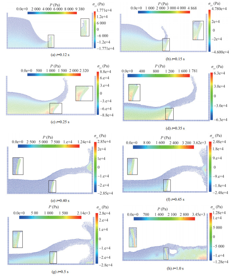Figure  25  Numerical simulation results of the test case: breaking-dam flow on an elastic baffle-fluid pressure field and stress component σ_yy in structure

Download: Full-Size Img

Figure 26 shows the horizontal displacement of the free left end of the elastic baffle U_x in terms of time in order to compare with the results of Walhorn et al. (2005) (FEM method), Idelsohn et al. (2008b) (PFEM method), and Rafiee and Thiagarajan (2009) (ISPH-WCSPH method). It is observed that the curves have a relative correspondence to the first peak. Walhorn's results predict the maximum displacement by about 18% less than the results of the present study. With passing the time, the results have been different. However, the second peak is relatively similar in time to other studies.

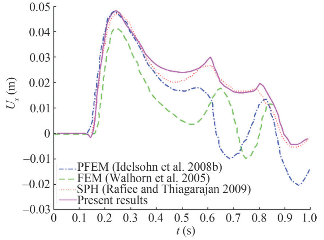Figure  26  Comparison between present results by ISPH-TLSPH model vs. numerical results (Idelsohn et al. 2008b; Walhorn et al. 2005; Rafiee and Thi-agarajan 2009) for time history of the horizontal displacement of the upper left corner of the baffle

Download: Full-Size Img

The force that the fluid exerts on the front wall, after passing through the elastic baffle, depends on the Young modulus of the baffle. By increasing the Young modulus, the amount of force applied to the wall decreases. The reason is that an elastic baffle with less flexibility makes more resistant to bending, therefore, more fluid momentum changes direction from horizontal to vertical, meaning that there is less horizontal momentum available in the flow when it impacts the side wall. The effect of the baffle on the amount of applied force on the front wall was studied by selecting different Young's modulus. Figure 27 shows the amount of applied force F_x on the wall in terms of time for three different Young's moduli, which is qualitatively concordant with the physics of the problem.

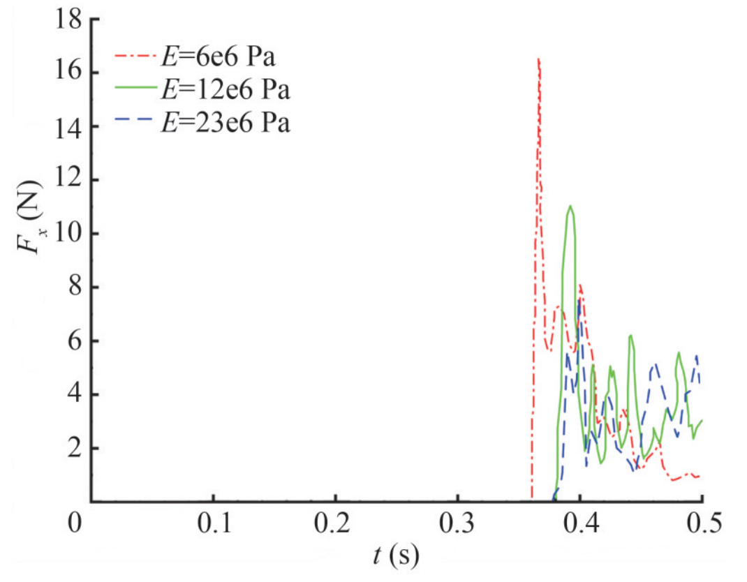Figure  27  Comparison of impact load for different Young modulus

Download: Full-Size Img

3.2.4   Flow in sloshing tank interacting with a clamped elastic baffle

The proposed ISPH-TLSPH FSI solver is applied in the simulation of sloshing in a rolling tank with a bottom clamped elastic baffle as compared with Idelsohn et al. (2008a). The initial configuration is illustrated in Figure 28. The fluid used is sunflower oil with density and kinematic viscosity of ρ_oil=917 kg/m³ and v_oil=5×10⁻⁵ m²/s, respectively. The elastic baffle with a density of ρ_b=1100 kg/m³ and Young's modulus of E=6 MPa, is clamped in the middle of the tank. A sinusoidal oscillation with a maximum amplitude of 4° and a period of t=1.211 s is prescribed to the tank.

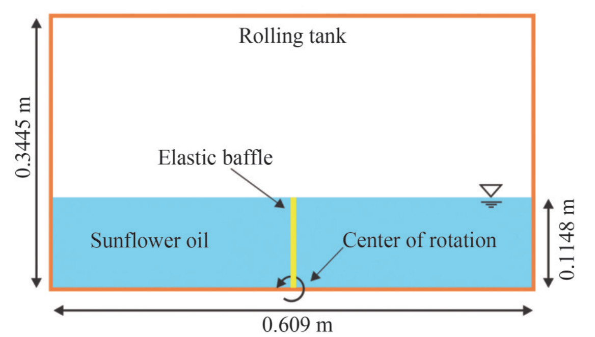Figure  28  Schematic sketch of sloshing with an elastic baffle clamped at the bottom of a rolling tank partially filled by oil (Idelsohn et al. 2008a)

Download: Full-Size Img

The experimental results are presented in Idelsohn et al. (2008a), inclusive of the local displacement of the tip of the elastic baffle and four photographs taken during the experiment to illustrate the deformation of the elastic body and the free-surface flow of fluid. Figure 29 shows qualitative comparisons between simulation snapshots and experimental photographs at the same instants. In general, the reproduced free-surface profiles and elastic baffle displacements well agree with the experiment. The positions of the wave trough and crest show good agreement between the simulation and the experiment. For time t=1.84 s, the free-surfaces matches with experimental result while structural deformation shows phase lag behind the expected. The minor observed discrepancies are expected to be due to an imprecise reproducibility of the working fluid's viscosity as well as considered assumptions in the mathematical model for structure. According to the presented figures, there is no un-physical gap in between fluid and structure and in specific, in the vicinity of fluid-structure interface, both the pressure and velocity divergence fields are well reproduced, thanks to the implemented fluidstructure coupling and the consistent particle shifting scheme.

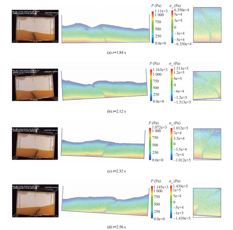Figure  29  Qualitative comparison between simulation snapshots and experimental photographs, obtained by Idelsohn et al. (2008a) corresponding to sloshing with elastic baffle clamped at bottom wall of a tank partially filled by oil.

Download: Full-Size Img

Figure 30 shows the time histories of displacements of elastic baffle's free end for comparison of simulation results with other published results (Idelsohn et al. 2008a; Khayyer et al. 2018a). The displacement curve shows periodic motion with respect to the sloshing tank as in the experiment. The good agreement in the amplitude of the displacement indicates that the coupling model can accurately perform in a long term simulation of viscous fluidelastic structure interaction.

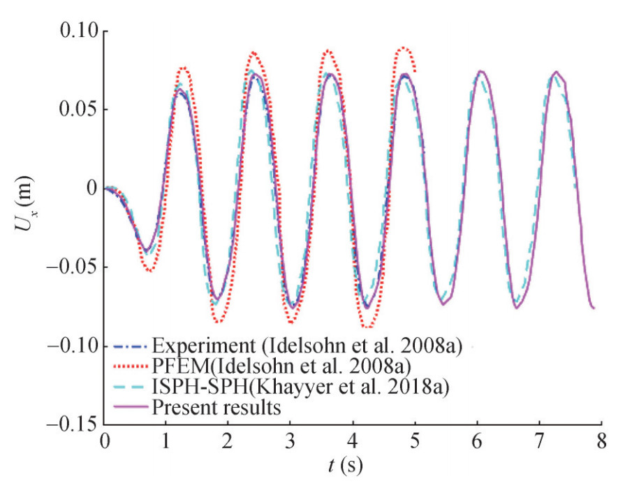Figure  30  Time histories of the displacement of the elastic baffle free end; present results by ISPH-TLSPH model vs. experimental results (Idelsohn et al. 2008a), PFEM by Idelsohn et al. (Idelsohn et al. 2008a) and ISPH-SPH (Khayyer et al. 2018a)-Sloshing with an elastic baffle clamped at the bottom wall of a tank

Download: Full-Size Img

4   Conclusion

The focus of this study is on the development, validation and application of a mesh-free computational method for simulating the flow of incompressible fluid in interacting with an elastic deformable structure. Hence, a numerical coupling model based on the SPH method was developed to investigate the fluid-structure interaction. The ISPH method was used to model the fluid in the determination of pressure to create a free-divergence velocity field, while the elastic structure was analyzed by TLSPH. In the ISPH method, the regular particle distribution is effective in the reproducing of a noise-free pressure field, to give a stable and accurate simulation. Xu et al. (2009) proposed a suitable algorithm for the particle displacement and correction of hydrodynamic variables to prevent numerical instabilities. However, due to incompleteness of the kernel domain of free-surface particles and adjacent to free-surface particles, numerical errors in their simulation lead to the lack of proper formation of the boundary of the fluid with the free surface. The proposed coupled method, without tuning a new parameter, results in a smooth and uniform pressure field in the fluid, as well as in the interface with the structure. The structure model was validated using two static and dynamic problems for the elastic structure and compared with its analytical results. Then, the numerical FSI coupled model combining with particle shifting scheme was evaluated by simulating several benchmark test cases in relation to the fluidstructure interaction. The simulation results in this study were compared with the analytical, experimental, and numerical results of other researchers. The good agreement of the results presented in this study with data from the other researchers showed the ability of the proposed model to simulate the phenomenon of fluid-structure interaction. The stability and capability of the coupled FSI-SPH solver by combining an ISPH scheme for fluid flows and a Total Lagrangian SPH (TLSPH) solver for elastic structures were demonstrated by comparing the flow profile of the fluid at the interface with the structure and the free surface with experimental results.

Appendix   Pseudo-code of the proposed algorithm