1   Introduction

In recent years, various countries have gradually started to attach importance to marine resources (Kim et al., 2014; Detweiller et al., 2007). However, some common media on land, such as electromagnetic waves and laser waves, are absorbed and attenuated significantly in the ocean (Hovem, 2007). Acoustic sensors are often used in underwater tasks since the sound wave is the only medium that can propagate a remote distance in marine environment. In general, acoustic sensors work in two ways: active mode and passive mode (Coraluppi et al., 2015). In the active mode, sensors detect the target by transmitting an acoustic signal of a certain frequency and receiving the echoes, while in the passive mode, hydrophones are only used to receive signals (Luo et al., 2018). Since the sensor consumes a lot of power and is prone to expose its position during transmission, the passive mode is preferable to be adapted for signal detection (Cui et al., 2014). However, with the development of acoustic concealment technology, many advanced countries have developed quiet submarines whose radiated noise is close to or lower than the marine background noise (Casey, 2007). Commonly used detection methods (such as detecting whether the amplitude of the received signal exceeds a predefined threshold) cannot detect such a weak signal (Chen et al., 2004). The radiated noise of the underwater target is mainly composed of periodic signals and appears as line spectra in the frequency domain (Wang and Shi, 2013). Therefore, it is an urgent problem that how to enhance the line spectrum of the underwater target and improve the SNR so as to be effectively detected, tracked, and identified (Siddagangaiah et al., 2016; Hu et al., 2011).

Conventional line spectrum detection methods such as FFT, short-time Fourier transform (STFT), and wavelet transform (WT) are not suitable for low SNR conditions (Abbate et al., 1997). Adaptive methods such as adaptive line spectrum enhancement (ALE) can separate the line spectrum without noise reference signal under low SNR conditions (Zhao et al., 2013). However, the method cannot adjust the convergence speed and steady-state error at the same time (Tufts et al., 1977; Luo et al., 2017). In recent years, some nonlinear detection methods such as high-order statistics (He et al., 2011), neural networks (Pan et al., 2010; West et al., 2017), chaotic oscillator (Chen et al., 2015; Li and Zhang, 2017), and entropy (Li and Chen, 2017) have been applied to the detection of underwater acoustic signals, but these methods are generally more complex or require prior information of signal frequency, which makes it difficult to applied in practice (Wang et al., 1999; Lv et al., 2009; Prince et al., 2015).

The Kalman filter (KF) algorithm and its variants are among the most popular estimation technique and have applications in almost all fields of technology (Izenman and Julian, 1988). In underwater acoustic environments, KF is often used in position determination, state estimation, and source localization (Luo et al., 2018; Kang et al., 2012). In addition, KF can also be used in signal detection. Su et al. combined KF and chaotic oscillators, firstly filtered the noise with KF, and then the Duffing chaotic oscillator is used to detect the weak harmonic signals in the strong fractional noise (Su et al., 2007). Pan et al. (2010) used the radial basis function neural networks to detect underwater acoustic weak signals, and KF is performed to reduce training errors during the optimization process (Pan et al., 2010). Moradi et al. used the adaptive Kalman filter to enhance the ECG signal (Moradi et al., 2014).

In the research of Kazemi et al. (2008), KF is used to detect and extract periodic noise in audio and biomedical signals. In addition, the audio and biomedical signals are filtered using KF models of different points in frequency range, and signal frequencies are estimated according to the amplitude of filtered signal. As a result, the authors solved the problem of detection of unknown frequency periodic noise. However, in marine environment, the frequency range is relatively large and SNR is lower, so the method would take a long time and have a large error.

In this paper, an algorithm combining KF and FFT-based spectrum analysis is proposed for enhancing the line spectrum of underwater signals under low SNR conditions. Firstly, the multi-frequency model is used to perform KF on the received signal, and then the frequency component of the signal is further determined according to the spectrum of the filtered signal. This process estimates the signal frequency so that the signal can be filtered more accurately and the line spectrum would be enhanced. This method solves the problem encountered by Kazemi et al. (2008) and is more suitable for underwater acoustic environment.

2   Kalman Filter Method

In general, there is some correlation between the latter and previous instant of signals. A simple model describing the correlation between samples is a first-order Gauss-Markov process. It is assumed that signals to be detected is a p-dimensional vector S(k); it can be expressed as:

Another assumption is that the M-dimensional observed data X(k) is the combination of the signal and the observed noise; it can be expressed as:

where k is the sampling moment, p×p matrix F is a state transition matrix, and p×M matrix D is a measurement matrix. v₁(k) and v₂(k) are independent random variables that exist during system transmission and observation. They are Gaussian white noise with a mean of zero and covariance matrices of Q₁ and Q₂. S(k) and X(k) are state vectors and measurement vectors, respectively. Equations (1) and (2) are the system and measurement equations of the KF algorithm.

In the following discussion, the minimum mean square error estimate of S(k) is denoted by Ŝ (k|k) and the minimum mean square error predictor of S(k) is denoted by Ŝ(k|k-1). The estimated error covariance matrix is represented as:

Also, the prediction error covariance matrix is represented as:

K(k) is the Kalman gain matrix during each iteration; then, the Kalman filter iterative algorithm is:

1) Initialize Ŝ(-1|-1) and M(-1|-1). The former can be set to zero and the latter can be set as a factor of identity matrix.

2) Calculate the minimum mean square error prediction value Ŝ(k|k-1) as:

3) Calculate the prediction error covariance matrix M(k|k-1) as:

4) Calculate the Kalman gain matrix K(k) as:

5) Correction to obtain the minimum mean square error estimate Ŝ(k|k) as:

6) Calculate the estimated error covariance matrix M(k|k) as:

7) Repeat 2)~6).

3   Mathematical Modeling for Line Spectrum Enhancement of Signal

In the following discussion, two cases of the known signal frequency and the unknown signal frequency are analyzed. When the signal frequency is known, the evolution of the deterministic signal is modeled, and the noise of other frequencies can be filtered out according to the established model, which achieves the effect of line spectrum enhancement. When the signal frequency is unknown, the signal frequency needs to be determined first, and then KF is used for line spectrum enhancement.

3.1   Single-Tone with Known Frequency

First, consider a simple case. It is assumed that the weak periodic signal to be detected is a single-tone signal with a known frequency, expressed as Asin(2πft + φ). After sampling the signal, it is expressed as Asin(2πfk / f_s + φ), where f_s is the sampling frequency. Then, the state vector is defined as:

According to the nature of the trigonometric function, S(k + 1) can also be expressed as:

Thus, the state transition matrix is defined as:

In Eq. (10), adding Acos(2πfk / f_s + φ) to the state vector is to make the transition relationship linear, so that modeling can be done using an ordinary KF without using an extend Kalman filter (EKF) or an unscented Kalman filter (UKF), thus reducing the error of the model. In this case, the measurement matrix is:

which indicates only the sine section can be received.

3.2   Multi-Tone with Known Frequency

Since the KF is good at processing multi-dimensional signals, the approach can be extended to a multi-frequency situation. When the signal to be detected contains n frequencies, it can be expressed as A₁sin(2πf₁t + φ₁) + A₂sin(2πf₂t + φ₂) + … + A_nsin(2πf_nt + φ_n), so the state vector is defined as:

Similarly, if F_i is defined as:

then, the state transition matrix is:

and the measurement matrix is:

which indicates only the sine sections can be received.

3.3   Unknown Frequencies

In practical applications, the frequency of the weak periodic signal to be detected is not accurately obtained, but sometimes we know the approximate range of the frequency (assumed to be [f_min, f_max]). Let the periodic signal be represented as a multi-frequency signal composed of the following frequencies [f₁, f₂, f₃…, f_n] (f_min ≤ f₁ < f₂ < … < f_n ≤ f_max), then perform KF on the signal using model in Section 3.2 and analyze the spectrum of the filtered signal. The KF model considers that there are some line spectra at [f₁, f₂, f₃…, f_n], thus filtering out noise at other frequency points. When the true frequencies of the signal happen to be some of the assumed frequencies, the spectrum of the filtered signal will produce a prominent peak here. The other case is that some signal frequency components are between two assumed frequencies. Since KF can adjust the Kalman gain K(k) by the prediction error covariance matrix M(k|k-1) in each iteration, the model can still perform effective filtering as long as the difference between the real frequency and one of the assumed frequencies is not very large. But when the true frequency component is far from the assumed frequencies on both sides, only increasing the value of the system noise variance Q₁ can compensate for the inaccuracy of the model. However, if Q₁ is too large, the filtering result will be inaccurate and fluctuating.

As a result, trade-offs are required when selecting assumed frequencies of the model before performing–KF. When the spacing of two assumed frequencies is too small, the peaks will overlap (in low SNR case) so the weak signal with the frequency between the two assumed values cannot be detected. On the other hand, when the spacing is too large, the true value may be too far from the assumed points and the amplitude will be small due to the model error, which is also difficult to detect.

Therefore, by expressing signals as a multi-frequency form in the frequency range, KF combined with FFT-based spectrum analysis could determine the frequency of signal. Performing KF on signals using the frequency information would enhance the line spectrum of signals, which facilitates the subsequent detection.

3.4   Parameter Selection

After determining the state vector, the transition matrix, and the measurement matrix, it is also necessary to give covariance matrices Q₁, Q₂ of system noise and measurement noise, and to initial estimated values Ŝ(-1|-1) and error covariance matrix M(-1|-1) to perform KF.

Typically, the variance of the system noise and measurement noise is chosen empirically. For example, when detecting a ship signal, it is assumed that the established model produces small errors, and the noise mainly comes from the measurement process. Therefore, the system noise variance and the measurement noise variance are set to 0.01 and 1, respectively. In addition, let the estimated values Ŝ(-1|-1) = 0 and error covariance matrix M(-1|-1) = I as the initial value. At this point, the KF algorithm can be used to filter the weak periodic signals.

4   Results and Discussion

In order to verify the line spectrum enhancement effect of the proposed algorithm on weak underwater acoustic signals, the method is performed on the computer simulation signal (generated by MATLAB) and the real ship signal, respectively.

4.1   Simulated Signals

It is assumed that the ship radiated signal to be detected is composed of a dual-frequency sinusoidal periodic signal and Gaussian white noise, and the signal is received after passing through a Rayleigh fading channel with five paths. The multipath delay vector is [0, 1.4, 1.8, 6.6, 7.2] ms, the average path gain vector is [0.4179, 0.2939, 0.09388, 0.07354, 0.04732], and maximum Doppler shift is 5 Hz. The channel parameters we used were from Deng's et al. (2009) paper and had been validated by comparing the output of the channel with the South China Sea test data.

The impulse and frequency responses of the Rayleigh channel are shown in Figures 1 and 2. The time domain waveform of the received signal is shown in Figure 3a, and the spectrum is shown in Figure 3b.

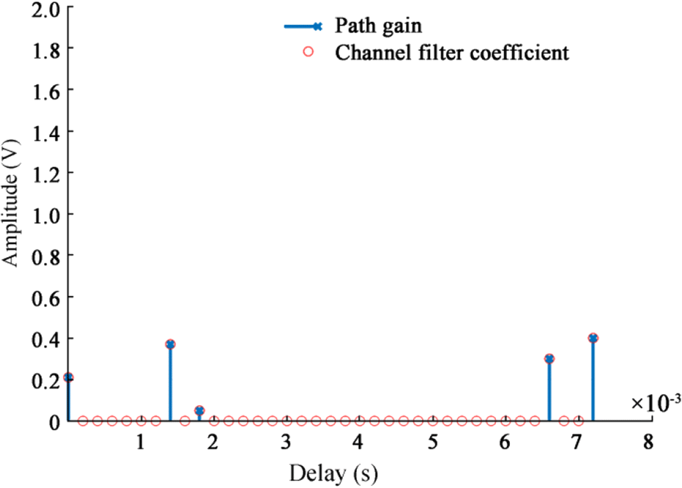Figure  1  Impulse responses of the Rayleigh channel

Download: Full-Size Img

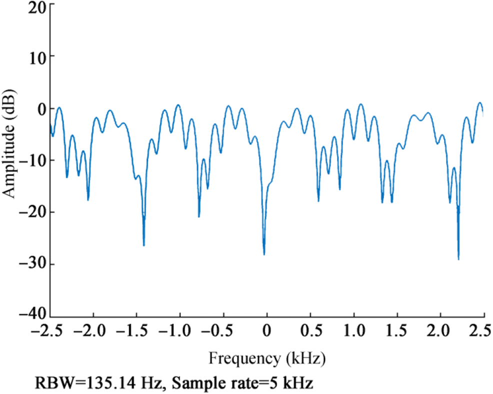Figure  2  Frequency responses of the Rayleigh channel

Download: Full-Size Img

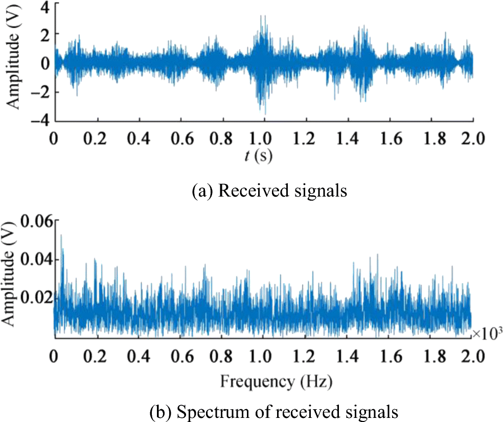Figure  3  Received signals and the spectrum

Download: Full-Size Img

Since the frequency information of the signal cannot be determined from Figure 3b, the frequency needs to be estimated first. In general, the frequencies of ships and submarines are mainly distributed at 0–2000 Hz. Therefore, let the simulated signal has a frequency range of 0–2000 Hz, and set [f₁, f₂, f₃…, f₆] = [0, 200, 400, …, 2000] be the filter parameters. The time and frequency domain waveform of the filtered signals are shown in Figure 4.

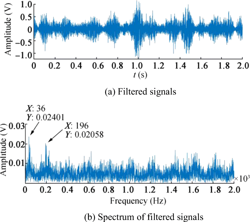Figure  4  Filtered signals and its spectrum

Download: Full-Size Img

From the spectrum of the filtered signals, it can be found that 36 Hz and 196 Hz may be the frequencies of signal. Thus, let [f₁, f₂] = [36196] be the filter parameters and let signals be filtered again by KF model, and time and frequency domain waveforms of the final filtered signal is shown in Figure 5.

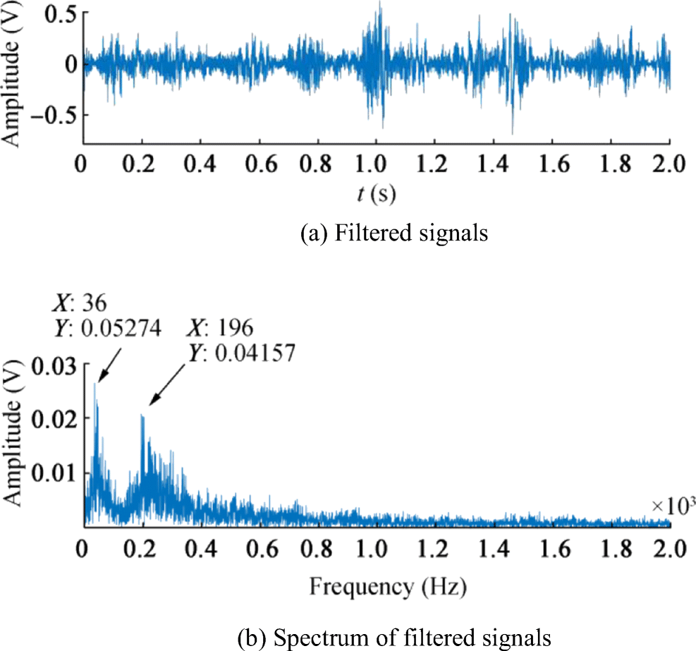Figure  5  Final filtered signals and its spectrum

Download: Full-Size Img

Comparing Figure 3b with Figure 5b, it can be found that line spectra of signals are detected and enhanced. If time domain waveforms of received and filtered signals are amplified, it can be seen from Figure 6 that the latter is smoother and some noise has been filtered out. The above results show that the proposed method can estimate the frequencies of signals and then enhance the line spectrum of the signals.

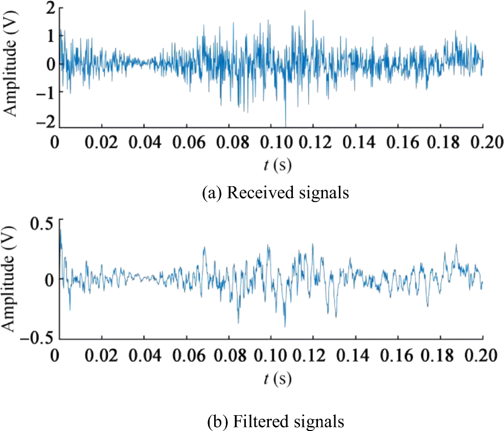Figure  6  Received signals and filtered signals

Download: Full-Size Img

It is worth mentioning that due to the Doppler effect, the frequency estimation may not be completely accurate. In fact, the periodic signal frequencies used in the simulation are 40 Hz and 200 Hz, but the filtering can still be performed effectively because of the small difference.

4.2   Ship Signals

After testing the simulated signal, a set of received ship signals was analyzed. During the experiment, the radiated noise of an unknown ship at the South China Sea was recorded by 16-element linear hydrophone array. The time domain waveform of received ship signal is shown in Figure 7a, and the frequency domain waveform is shown in Figure 7b.

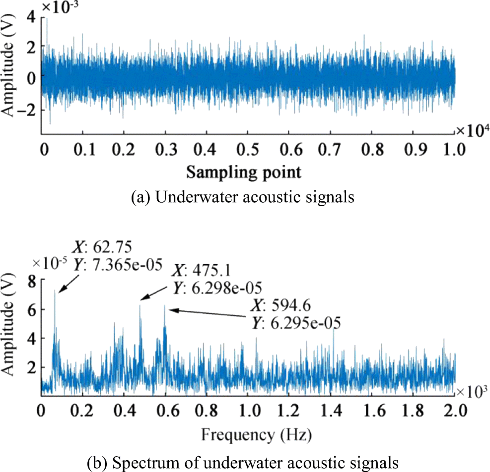Figure  7  Samples of ship signals and its spectrum

Download: Full-Size Img

From Figure 7b, it could be found that the amplitudes of the three frequency components are slightly higher than the average, 62.75, 475.1, and 594.6 Hz. Thus, we set [f₁, f₂, f₃] = [62.75, 475.1, 594.6] as the filter parameters and use KF to enhance the line spectra. The time domain waveform and frequency of filtered signals are shown in Figure 8.

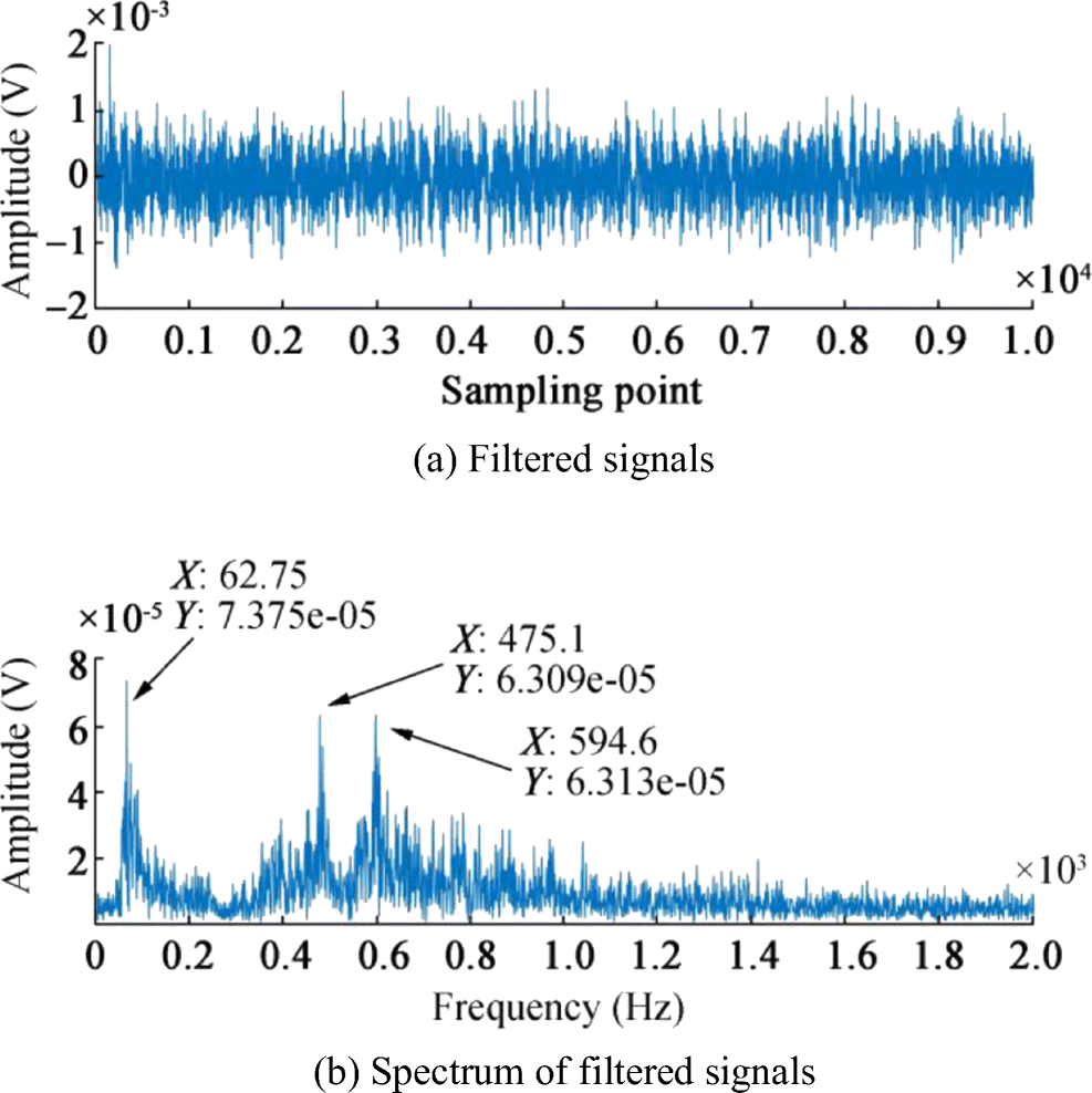Figure  8  Filtered signals and its spectrum

Download: Full-Size Img

Comparing Figure 7b with Figure 8b, it can be found that the noise at other frequencies are filtered out, and the line spectra of the signals are enhanced. The time domain waveform comparison of the ship signals and the filtered signal is shown in Figure 9. It can be found that the filtered signal has less clutter and the waveform is smoother.

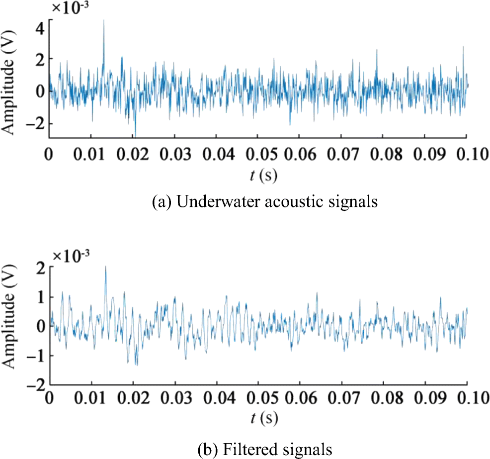Figure  9  Ship signals and filtered signals

Download: Full-Size Img

5   Conclusion

This paper describes the line spectrum enhancement of underwater acoustic signals based on Kalman filter. Because the line spectrum of the underwater acoustic target is expressed as a periodic signal in the time domain, a linear transfer model can be established for underwater acoustic signals and then Kalman filtering can be used. This paper established a model in several different cases of single-tone with known frequency, multi-tone with known frequency, and unknown frequencies. Among them, when the signal frequency is unknown, Kalman filtering is performed on the signal using some assumed frequencies in the signal frequency range to estimate the signal frequency; when the signal frequency is known or already estimated, the signal can be filtered more accurately to achieve the effect of line spectrum enhancement. Experiments on simulated signals and ship signals are conducted in this paper, and the results show that the line spectra of the underwater acoustic target are enhanced and the SNR are improved in both cases. The filtering achieves satisfactory results and proves the effectiveness of this method. Enhancements to the line spectra of underwater targets could be used to improve the detection ability of underwater detection systems and weapon systems.