Numerical Study on the Hydrodynamic Performance of Antifouling Paints
https://doi.org/10.1007/s11804-020-00130-w
-
Abstract
This study presents a simple numerical method that can be used to evaluate the hydrodynamic performances of antifouling paints. Steady Reynolds-averaged Navier-Stokes equations were solved through a finite volume technique, whereas roughness was modeled with experimentally determined roughness functions. First, the methodology was validated with previous experimental studies with a flat plate. Second, flow around the Kriso Container Ship was examined. Lastly, full-scale results were predicted using Granville's similarity law. Results indicated that roughness has a similar effect on the viscous pressure resistance and frictional resistance around a Reynolds number of 107. Moreover, the increase in frictional resistance due to roughness was calculated to be approximately 3%-5% at the ship scale depending on the paint.Article Highlights• The surface condition of a ship could be successfully modeled by modifying wall functions.• The effect of surface roughness on the viscous resistance components of a ship was investigated via computational fluid dynamics (CFD).• Full-scale results for the same ship was predicted using the inner wall similarity law.• Further CFD simulations were performed using a container ship model.• A verification study was conducted using previous experimental results. -
1 Introduction
Maritime transportation has become one of the most important elements of the global trade because of its economic advantages, which have been increasing with the increasing size of ships. An ultra large container vessel can carry more than 15000 twenty-foot containers, whereas the loading capacity of an ultra large crude carrier can reach up to 550 000 DWT (IMO 2009). According to UNCTAD (2018), ships carry 80%-90% of the goods. Meanwhile, concern on air pollution is increasing due to shipping activities and the use of fossil fuels. Thus, global regulations related to greenhouse gas (GHG) emissions are being strengthened nowadays. With the Energy Efficiency Design Index and the Ship Energy Efficiency Management Plan, IMO aims to reduce CO2 emissions. GHG emissions have been predicted to decrease by 10%-17% until 2020 and 19%-26% until 2030 (IMO 2011). In brief, the energy efficiency of ships is a major priority for global regulations and the need for green shipping forces companies to reduce fuel consumption.
An accurate assessment of the hydrodynamic performance of ships is crucial to achieve energy-efficient designs and reduce fuel consumption. Such assessment requires deep knowledge about resistance components and their interrelations. The skin friction resistance of a ship generally forms the biggest portion of its total resistance, and it may further dramatically increase due to the roughness condition of the outer surface (Lackenby 1962). Ships are under a continuous thread of fouling. Biological attacks and chemical corrosions at the outer surface of ships considerably affect its hydrodynamic performance. Even though fouling can be prevented or decelerated in several ways, the most common and effective one is the application of antifouling paints (Candries et al. 2001). Consequently, there have been continuous developments of the antifouling paints due to the fact that the resistance, and the fuel consumption of ships is highly sensitive to its surface conditions. Recently, researchers have been searching for a simple method to evaluate the success of different paints (Atlar et al. 2018; Demirel 2018; Demirel et al. 2014, 2017; Unal 2012; Unal 2015; Yeginbayeva 2017). However, such a method is difficult to develop because of the irregularity of paint-coated surfaces. In addition, roughness changes the flow characteristic at the wake region, as well as in the boundary layer. Thus, flat plate results are not enough to understand the physics. Full-scale trials might be helpful to understand the problem. However, trials are costly and difficult; thus, the literature is limited (Hundley and Tate 1980; Haslbeck and Bohlander 1992).
Computational fluid dynamics (CFD) applications provide a new tool to simulate the rough flow around three-dimensional bodies (Demirel et al. 2014, 2017; Khor and Xiao 2011; Haase et al. 2016; Rushd et al. 2018; Farkas et al. 2018; Song et al. 2019). Generally, surface roughness is modeled with a function that has a downward shift at the normalized velocity profile. However, flat plate experiments are indispensable for obtaining enough roughness functions. Additionally, such research mostly focuses on the frictional or wave resistance of the vessel and ignores the viscous pressure component of the total resistance of the ship.
This study presents a simple numerical method to evaluate the hydrodynamic performance of different antifouling paints. The experimental results of Schultz (2004) are used to validate the presented methodology. The main goal of this study is to investigate the effect of hull roughness on viscous pressure resistance and subsequently the form factor of the vessel. Therefore, the three-dimensional flow around the Kriso Container Ship (KCS) at the model scale is analyzed. Lastly, full-scale predictions are made using Granville's (1958) extrapolation scheme. The flat plate results are in good agreement with the experimental results, indicating that the presented methodology is beneficial to the investigation of the flow around antifouling paint-coated ships.
2 Turbulent Boundary Layer
When a ship in motion is examined closely, a thin turbulent flow region, which extends along the vessel, is observed. Thus, the concept of turbulent boundary layer is important for understanding such flows. The forward end of a vessel has a small region where the flow is laminar. Then, it becomes turbulent as the local Reynolds number increases. The third region between the laminar and turbulent portions is called the transition region. At the typical Reynolds numbers for ship flows, laminar portion is so small that flow can be assumed as fully turbulent (Bertram 2000).
In contrast to laminar boundary layers, turbulent boundary layers are beneficial to examine under several discrete regions because the flow displays different characteristics depending on the distance from the wall. Turbulent boundary layers comprise an inner and an outer region. The inner region can be divided into a viscous sublayer and a log-law region. Typically, the normalized mean velocity (U+) in this region is expressed by:
$$ {U}^{+}=f\left({y}^{+}\right) $$ (1) where y+ is the nondimensional normal distance from the wall; these terms can be obtained from:
$$ {U}^{+}=\frac{U}{U_{\tau }}\kern1em $$ (2) $$ {y}^{+}=\frac{y{U}_{\tau }}{\nu}\kern0.5em $$ (3) where U is the mean velocity, y is the normal distance from the wall, and ν is the kinematic viscosity of the fluid. Uτ is the friction velocity, which is defined as:
$$ {U}_{\tau }=\sqrt{\frac{\tau_w}{\rho }} $$ (4) where τw is the shear stress at the wall surface, and ρ is the density of the fluid. In the region very close to the wall, where y+ < 5, the normalized mean velocity profile shows a linear dependence, which can be obtained directly from Newton's theorem of the viscous fluid (Schlichting 1979). This region is called a linear sublayer.
$$ {U}^{+}={y}^{+} $$ (5) The log-law region comprises the region between 30 < y+ < 300, and the normalized mean velocity can be given by following relation (Schlichting 1979):
$$ {U}^{+}=\frac{1}{\kappa}\ln {y}^{+}+B $$ (6) where κ is the von Karman constant, and B is another constant. Figure 1 shows a typical mean velocity profile in a turbulent boundary layer (Schultz 2004).
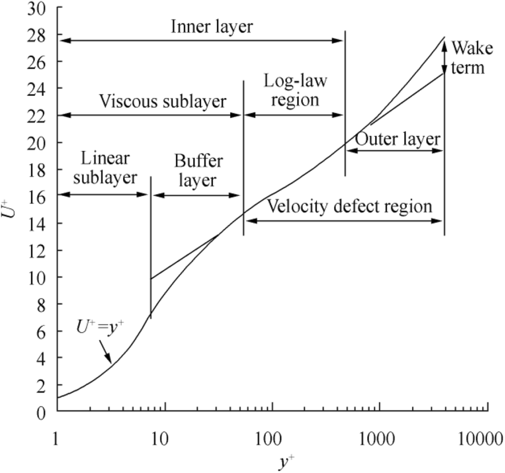 Figure 1 Mean velocity profile in a turbulent boundary layer (Schultz 2004)
The inner layer is very sensitive to the surface condition, whereas roughness has no direct effect on the characteristics of the outer layer (Schetz and Bowersox 2011). When all roughness elements are in the viscous sublayer, roughness does not change the flow topology, and the flow is hydraulically smooth. When only some of the elements exceed the viscous sublayer, some eddies and separations occur behind these elements, and flow is called transitionally rough. When these additional eddies and separations become dominant, the flow is called fully rough. Figure 2 shows the flow regimes depending on the roughness height. The key parameter of roughness is thought to be the roughness height, which is normalized similar to the nondimensional distance.
$$ {k}^{+}=\frac{k{U}_{\tau }}{\nu}\kern0.5em $$ (7) $$ A{U}^{+}\left({y}^{+},{k}^{+}\right)=\frac{1}{\kappa}\ln {y}^{+}+B-{\Delta U}^{+}\left({k}^{+}\right) $$ (8) where k+ is called the roughness Reynolds number, and k is the characteristic roughness height.
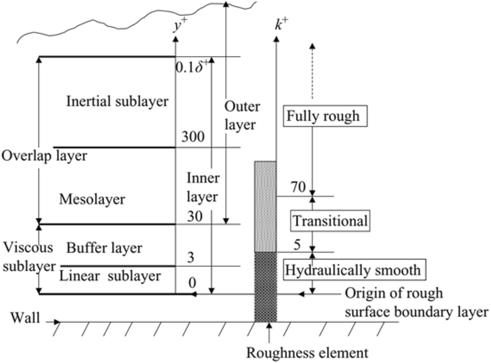 Figure 2 Roughness regimes depending on the roughness height (Cal et al. 2009)
With the existence of roughness, the velocity profile at the inner region changes with k+ and y+. The normalized mean velocity profile can be expressed similar to Eq. (6), with an additional term called roughness function (ΔU+) (Clauser 1954).
The physical meaning of Eq. (8) is that roughness causes only a parallel downward shift at the normalized mean velocity profile, which depends only on the roughness Reynolds number. The decrease in the mean velocities causes an increase in frictional resistance. Additionally, the roughness function can only be experimentally obtained particularly for irregular rough surfaces. Figure 3 shows the downward shift of the normalized mean velocity profile due to roughness.
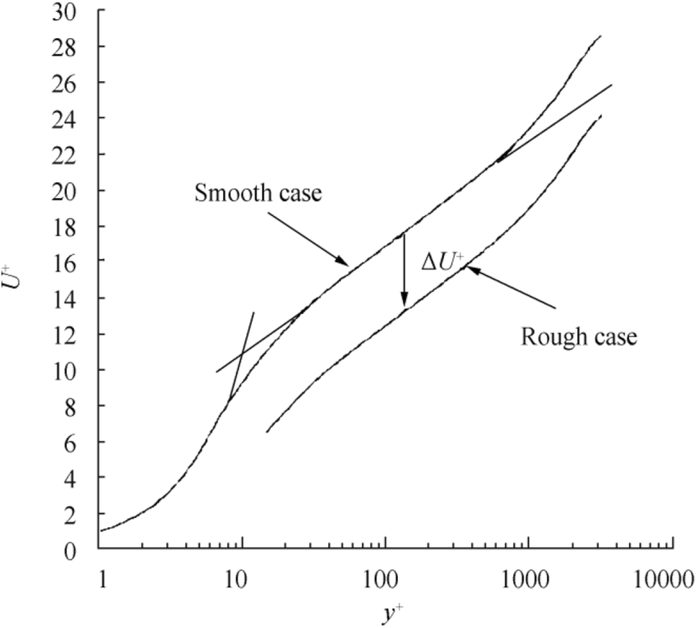 Figure 3 Downward shift due to roughness (Demirel et al. 2014)
3 Mathematical Model
Flows are modeled with steady incompressible Reynolds-averaged Navier-Stokes (RANS) equations. The continuity and momentum equations are given as (Wilcox 2006):
$$ \frac{\partial \overline{u_i}}{\partial {x}_i}=0 $$ (9) $$ \frac{\partial }{\partial {x}_j}\left(\rho \overline{u_i}\overline{u_j}+\rho \overline{u_i^{\prime }{u}_j^{\prime }}\right)=-\frac{\partial \overline{p}}{\partial {x}_i}+\frac{\partial \overline{\tau_{ij}}}{\partial {x}_j} $$ (10) where $ \overline{u_i} $ is the averaged velocity components, $ \rho \overline{u_i^{\prime }{u}_j^{\prime }} $ is Reynolds stress terms, $ \overline{p} $ is the averaged pressure, and $ \overline{\tau_{ij}} $ is the averaged stress tensor components. For an isotropic Newtonian fluid, $ \overline{\tau_{ij}} $ can be given as:
$$ \overline{\tau_{ij}}=\mu \left(\frac{\partial \overline{u_i}}{\partial {x}_j}+\frac{\partial \overline{u_j}}{\partial {x}_i}\right) $$ (11) where μ is the dynamic viscosity of the fluid.
The shear-driven two-layer (Wolfstein 1969) realizable k-ε model (Shih et al. 1995), which is based on the Boussinesq hypothesis (Tennekes and Lumley 1972), is used to model Reynolds stress terms. Transport equations of the model are given as:
$$ \frac{\partial k}{\partial t}+{U}_j\frac{\partial k}{\partial {x}_j}=-\overline{u_i^{\prime }{u}_j^{\prime }}\frac{\partial {U}_i}{\partial {x}_j}-{\varepsilon}_{ij}+\frac{\partial }{\partial {x}_j}\left[\left(\upsilon +\frac{\upsilon_T}{\sigma_k}\right)\frac{\partial k}{\partial {x}_j}\right] $$ (12) $$ \frac{\partial \varepsilon }{\partial t}+{U}_j\frac{\partial \varepsilon }{\partial {x}_j}={C}_1S{\varepsilon}_{ij}-{C}_{\varepsilon 2}\frac{\varepsilon^2}{k+\sqrt{\nu \varepsilon}}+\frac{\partial }{\partial {x}_j}\left[\left(\upsilon \\ +\frac{\upsilon_T}{\sigma_{\varepsilon }}\right)\frac{\partial \varepsilon }{\partial {x}_j}\right] $$ (13) In Eqs. (12) and (13), k is the turbulent kinetic energy, ε is the turbulent dissipation rate, and S is the modulus of the mean stress tensor. υT is called kinematic eddy viscosity, which is given as:
$$ {\upsilon}_T={C}_{\mu}\frac{k^2}{\varepsilon } $$ (14) Cμ is calculated from Eqs. (15)-(20).
$$ {C}_{\mu }=\frac{1}{A_0+{A}_s\frac{k{U}^{\ast }}{\varepsilon }} $$ (15) $$ {A}_0=4.04,{A}_S=6\cos \phi $$ (16) $$ \phi =\frac{1}{3}{\cos}^{-1}\left(\sqrt{6}W\right) $$ (17) $$ W=\frac{S_{ij}{S}_{jk}{S}_{ki}}{{\overset{\sim }{S}}^3} $$ (18) $$ \overset{\sim }{S}=\sqrt{S_{ij}{S}_{ij}}\kern0.5em $$ (19) $$ {S}_{ij}=\frac{1}{2}\left(\frac{\partial {u}_j}{\partial {x}_i}+\frac{\partial {u}_i}{\partial {x}_j}\right) $$ (20) The empirical constants of the model are given as follows:
$$ {C}_{\varepsilon 1}=1.44,{C}_{\varepsilon 2}=1.9,{\sigma}_k=1,{\sigma}_{\varepsilon }=1.2 $$ (21) The continuity, momentum, and turbulent transport equations are solved with a finite volume technique that uses a segregated algorithm (Wilcox 2006). A second-order upwind scheme is used for the discretization of the viscous terms, whereas a second-order central difference scheme is used for convective terms (Wilcox 2006). Pressure field is solved with the SIMPLE algorithm (Patankar and Spalding 1972). Star CCM+ software is used to solve the abovementioned equations.
4 Wall Function
The wall function approach with high y+ values is used to link the viscous sublayer to the log-law region. This approach requires that the near cells, which are adjacent to the wall, lie within the log-law region. The normalized velocity distribution is modeled as follows (CD-ADAPCO 2011):
$$ {U}^{+}=\frac{1}{\kappa}\ln \left(\frac{E{y}^{+}}{f}\right) $$ (22) where E is called the wall function coefficient, and f is called the roughness coefficient. Eq. (22) is completely identical to Eq. (8). A direct relationship exists between f and roughness function, and its value depends on the roughness Reynolds number. Depending on the flow regime, f is defined as follows (CD-ADAPCO 2011):
$$ f=\left\{\begin{array}{ccc}1& \to & {k}^{+} \lt {k}_{\mathrm{sm}}^{+}\\ {}{\left[A\left(\frac{k^{+}-{k}_{\mathrm{sm}}^{+}}{k_r^{+}-{k}_{\mathrm{sm}}^{+}}\right)+C{k}^{+}\right]}^a& \to & {k}_{\mathrm{sm}}^{+}\le {k}^{+}\le {k}_r^{+}\\ {}A+C{k}^{+}& \to & {k}_r^{+} \lt {k}^{+}\end{array}\right. $$ (23) $$ a=\sin \left[\frac{\pi}{2}\frac{\log \left({k}^{+}/{k}_{\mathrm{sm}}^{+}\right)}{\log \left({k}_r^{+}/{k}_{\mathrm{sm}}^{+}\right)}\right] $$ (24) The above expressions are a slightly expanded version of the model given by Cebeci and Bradshaw (1977). When $ {k}^{+} \lt {k}_{\mathrm{sm}}^{+} $, the flow is hydraulically smooth; when $ {k}_r^{+} \lt {k}^{+} $, the flow is fully rough. This model assumes that the flow develops over closely packed sands with the default values of $ {k}_{\mathrm{sm}}^{+}=2.25 $, kk+ = 90, A = 0, and C = 0.253. In this study, the same model is applied for sandpaper cases, whereas a different model is adopted for antifouling paint cases on the basis of Schultz's (2004) suggestions. For antifouling paint cases, f is chosen such that Grigson's (1992) roughness function is satisfied.
$$ {\Delta U}^{+}=\frac{1}{\kappa}\ln \left(1+{k}^{+}\right) $$ (25) For irregular surfaces, such as antifouling coatings, the determination of the characteristic roughness height is also crucial and should be experimentally determined on the basis of the surface statistics and measured velocity profiles. In this study, the characteristic roughness heights are taken as 17% of the averaged amplitude of roughness (Ra) for the antifouling paint cases and 75% of the maximum peak to trough height (Rt), as suggested by Schultz (2004). Surface statistics are given in Table 1, where Rq denotes the root mean square roughness height (Schultz 2004). The values of E and κ are taken as 9 and 0.42, respectively.
Table 1 Roughness statistics of the surfaces (Schultz 2004)Test surface Ra Rq Rt Silicon 1 12 ± 2 14 ± 2 66 ± 7 Silicon 2 14 ± 2 17 ± 2 85 ± 8 Ablative copper 13 ± 1 16 ± 1 83 ± 6 SPC copper 15 ± 1 18 ± 1 97 ± 10 SPC TBT 20 ± 1 24 ± 2 129 ± 9 60-Grit SP 126 ± 5 160 ± 7 983 ± 89 220-Grit SP 30 ± 2 38 ± 2 275 ± 17 5 Geometries and Boundary Conditions
The plate dimensions used in the validation studies are shown in Figure 4. The thickness of the plate was simply neglected because it is very small compared with its length and width. Computations were performed using two different flow speeds, which correspond to the Reynolds number of 2.8 × 10⁶ and 5.5 × 10⁶.
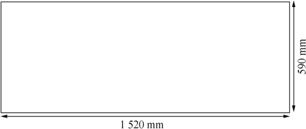 Figure 4 Dimensions of the plate
Figure 5 shows the computational and boundary conditions for the numerical analysis of the flat plate cases. A volume in the form of a rectangular prism was selected, and a right-handed Cartesian coordinate system was applied. The origin of the system was located at the intersection of the forward end and symmetry axis of the plate, where the positive x axis shows the after part of the length of the plate, and the positive z axis shows the upwards. On the basis of the experiments of Schultz (2004), the upstream boundary was located at 1 L in front, the downstream boundary was located at 4 L at the back, and the side boundary was located at 2 L from the plate, where L denotes the length of the plate. The bottom boundary was located at 1.5 L below the plate. The velocity inlet condition was applied at the upstream, and the pressure outlet condition was applied at the downstream. The wall condition with zero shear stress was applied at the side, top, and bottom boundaries.
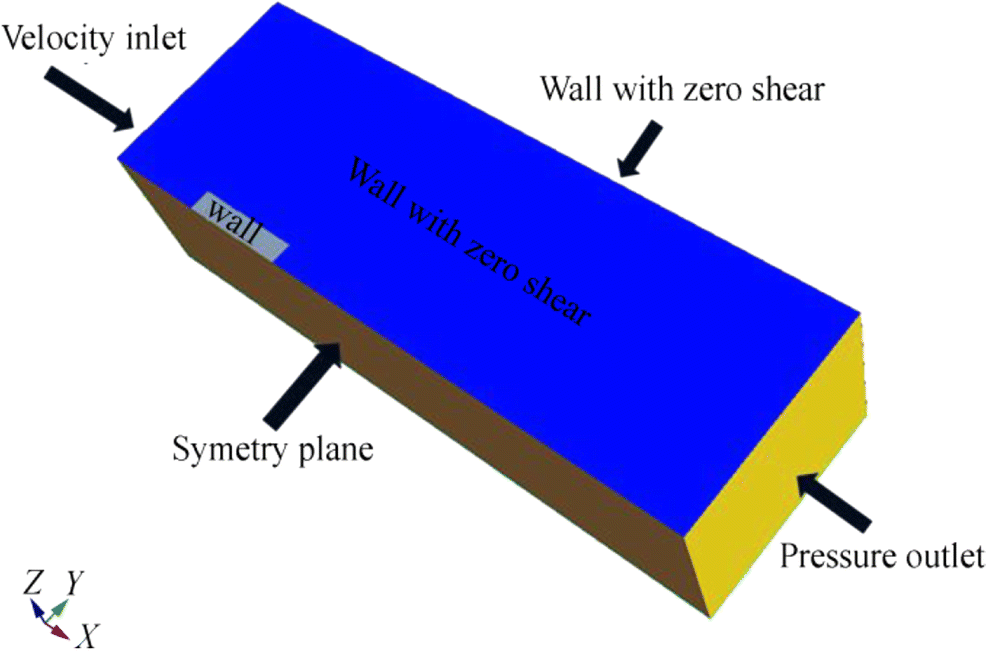 Figure 5 Computational domain and boundary conditions for the flat plate
Figure 6 shows the surface geometry of the KCS model. Analysis was conducted at the model scale. The general characteristics of the geometry at model and ship scales are given in Table 2. The computational domain and the boundary conditions of the KCS model are shown in Figure 7.
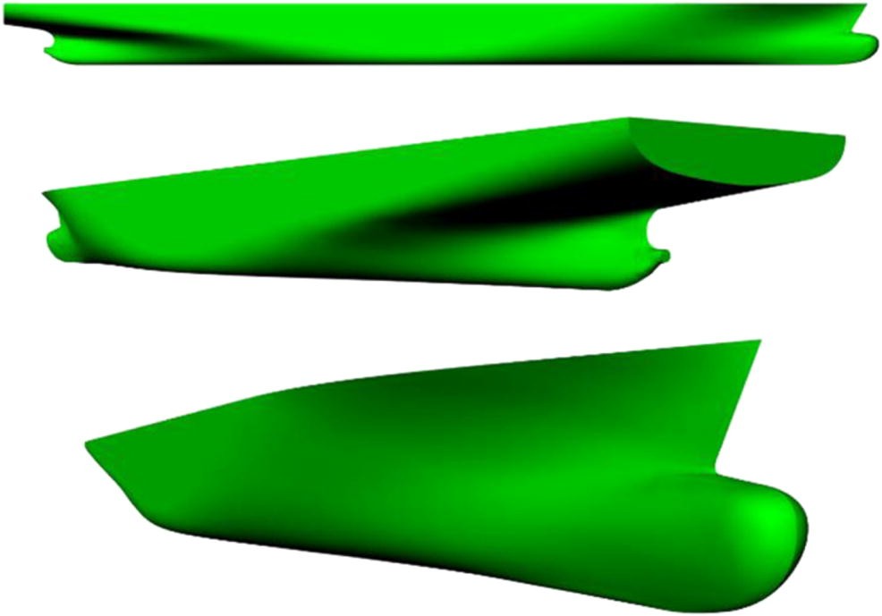 Figure 6 Geometry of KCSTable 2 General characteristics of KCS
General characteristics Ship scale Model scale Scale - 31.60 Length between perpendiculars (m) 230 7.278 Beam (m) 32.2 1.019 Draught (m) 10.8 0.341 Depth (m) 19 0.601 Block coefficient 0.65 0.650 Wetted surface area (m2) 9424 6.437 Displacement (m3) 52 030 1.648 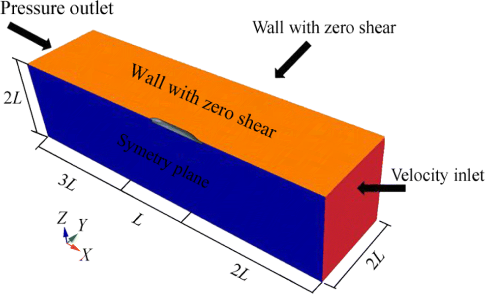 Figure 7 Computational domain and boundary conditions for KCS
6 Mesh Generation and Grid Dependence
For the flat plate cases, all analyses were performed with structured meshes due to the simplicity of the geometry. Numerical uncertainties due to discretization were estimated using Roache's (1998) method of grid convergence index (GCI). The detailed description of the method is given in Çelik et al. (Celik et al. 2008).
Figure 8 shows the general structure of the mesh used for the flat plate analysis. Three meshes with different densities were created for the GCI calculations. For all cases, average wall y+ values were kept at approximately 50. GCI calculations were only performed under smooth surface conditions.
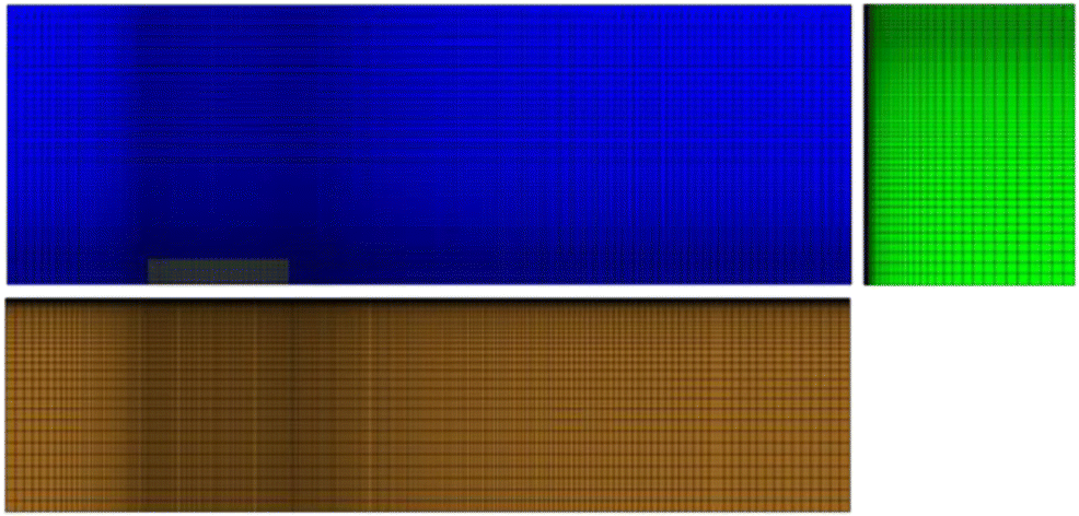 Figure 8 Structured grid for flat plate analysis
The general characteristics of the grids and the calculated frictional resistance coefficient values are summarized in Table 3. The corresponding Reynolds number for the GCI analysis was 2.8 × 10⁶. After the generation of coarse grids, cell densities at the x, y, and z directions were increased systematically with a refinement factor of $ \sqrt{2} $.
Table 3 Grid structures and frictional resistance coefficients for flat plateCell density Cell number (i × j × k) Cf (CFD) Cf (EFD) RD% Coarse (N3) 199 × 58 × 35 0.003552 0.003605 1.47 Medium (N2) 281 × 82 × 50 0.003548 0.003605 1.58 Fine (N1) 398 × 116 × 70 0.003550 0.003605 1.53 The results of the GCI calculations are summarized in Table 4. The results indicate that the numerical uncertainty due to discretization is 0.65%. Further analysis was performed using a medium mesh because the relative difference of the medium and fine meshes was below 0.1%.
Table 4 GCI calculation results for flat plateN1, N2, N3 3 231 760, 1 152 100, 403 970 r21, r32 $\sqrt{2} $ ϕ1 0.003550 ϕ2 0.003548 ϕ3 0.003552 p21 0.287 ${\phi}_{21}^{\mathrm{ext}} $ 0.003568 ${\mathrm{GCI}}_{\mathrm{fine}}^{21} $ 0.65% In contrast to the flat plate, KCS has a complex geometry, with high surface curvatures at the bow and stern of the ship. For this reason, unstructured meshes and meshes with high resolutions were used to model the near ship region and the bow and stern of the ship, respectively. Meshes were created using the mesh generation tool of Star CCM+. Figure 9 shows a 3D view of the generated mesh for the KCS cases.
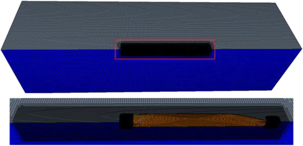 Figure 9 3D view of the KCS mesh
Four meshes with different densities were created to estimate the uncertainty due to discretization. The GCI calculations were performed with the corresponding Froude number of 0.26 and Reynolds number of 1.402 × 10⁷. The general characteristics of the meshes and the obtained frictional resistance coefficients are summarized in Table 5. For comparison purposes, the frictional resistance coefficients calculated using the ITTC (1957) formula are also added to the table.
Table 5 Grid Structures and frictional resistance coefficients for KCSCell density Cell number Cf (CFD) Cf (ITTC-1957) %RD Coarse (N4) 291 113 0.002667 0.00283 4.03 Medium (N3) 635 417 0.002754 0.00283 0.90 Fine (N2) 1 440 643 0.002748 0.00283 1.11 Finest (N1) 3 268 535 0.002773 0.00283 0.22 The GCI calculation results are shown in Table 6. Results indicate that the discretizational uncertainty of the fine grid is 0.01%, whereas that for the finest grid uncertainty is calculated as 0.25%. The fine grid was chosen for further analysis.
Table 6 Grid Structures and frictional resistance coefficients for KCSN1, N2, N3, N4 3 268 535, 1 440 643, 635 417, 291 113 r21, r32, r43 1.314, 1.313, 1.297 ϕ1 0.002773 ϕ2 0.002748 ϕ3 0.002754 ϕ4 0.002667 p21 6.22 p32 10.63 ${\phi}_{21}^{\mathrm{ext}} $ 0.002779 ${\phi}_{32}^{\mathrm{ext}} $ 0.002748 ${\mathrm{GCI}}_{\mathrm{fine}}^{32} $ 0.01% ${\mathrm{GCI}}_{\mathrm{finest}}^{21} $ 0.25% 7 Results and Discussion
7.1 Flat Plate Results
he comparative results of the Cf values obtained by the CFD study and the EFD study of Schultz (2004) are shown in Tables 7 and 8, respectively. The Cf values calculated by Demirel et al. (2014) were also added to the tables for comparison purposes. The relative differences for all cases were found to be less than 3%, except for the 60-grit SP surface. On the 60-grit SP surface, the results estimated from CFD analysis were significantly less than the experimental results. This discrepancy could be explained by the fact that the roughness of this surface is significantly higher than the others. On the surfaces with high roughness, the downward shift of the normalized mean velocity profile is also high, thus causing a singularity in the calculations when the adjacent cell is too close to the wall boundary (see Figure 3). The Star CCM+ software uses the roughness restriction option to overcome this singularity and reduces the surface roughness when singularity occurs. As a result, when the distance of the first cell adjacent to the wall surface is not large enough, the frictional resistance values are considerably underpredicted. This issue should be considered in studies where surface roughness is modeled using wall function approaches (CD-ADAPCO 2011).
Table 7 Comparative Cf Values at Re = 2.8 × 10⁶Surface Cf (×103) (Current Study) Cf (×103) (EFD) Cf (×103) (Demirel et al. 2014) RD% Smooth 3.548 3.605 3.632 1.58 Silicon 1 3.647 3.666 3.715 0.52 Silicon 2 3.662 3.663 3.729 0.03 Ablative copper 3.655 3.701 3.722 1.24 SPC copper 3.669 3.723 3.736 1.45 SPC TBT 3.703 3.783 3.776 2.11 60-grit SP 5.077 6.057 N/A 16.2 220-grit SP 4.317 4.258 N/A 2.40 Table 8 Comparative Cf values at Re = 5.5 × 10⁶Surface Cf (×103) (Current Study) Cf (×103) (EFD) Cf (×103) (Demirel et al. 2014) RD% Smooth 3.174 3.226 3.185 1.61 Silicon 1 3.315 3.374 3.460 1.75 Silicon 2 3.335 3.426 3.481 2.66 Ablative Copper 3.325 3.401 3.470 2.23 SPC Copper 3.344 3.438 3.491 2.73 SPC TBT 3.392 3.500 3.551 3.09 60-grit SP 4.486 5.954 N/A 24.7 220-grit SP 4.360 4.252 N/A 2.54 Figures 10 and 11 show the shear stress distributions on the surfaces calculated at Re = 2.8 × 10⁶. The distribution of the roughness Reynolds number can also be obtained from the shear stress values due to the proportionality of the shear stress. As expected, the local shear stress values show a parallel increase with the surface roughness and take the largest value on a line near the forward end of the plate. This result is expected, considering that the roughness has a great effect on the shear stress where the boundary layer is thinner. Local shear stress values on painted surfaces generally range from 3 Pa to 15 Pa, whereas sanded surfaces have values reaching up to 40 Pa.
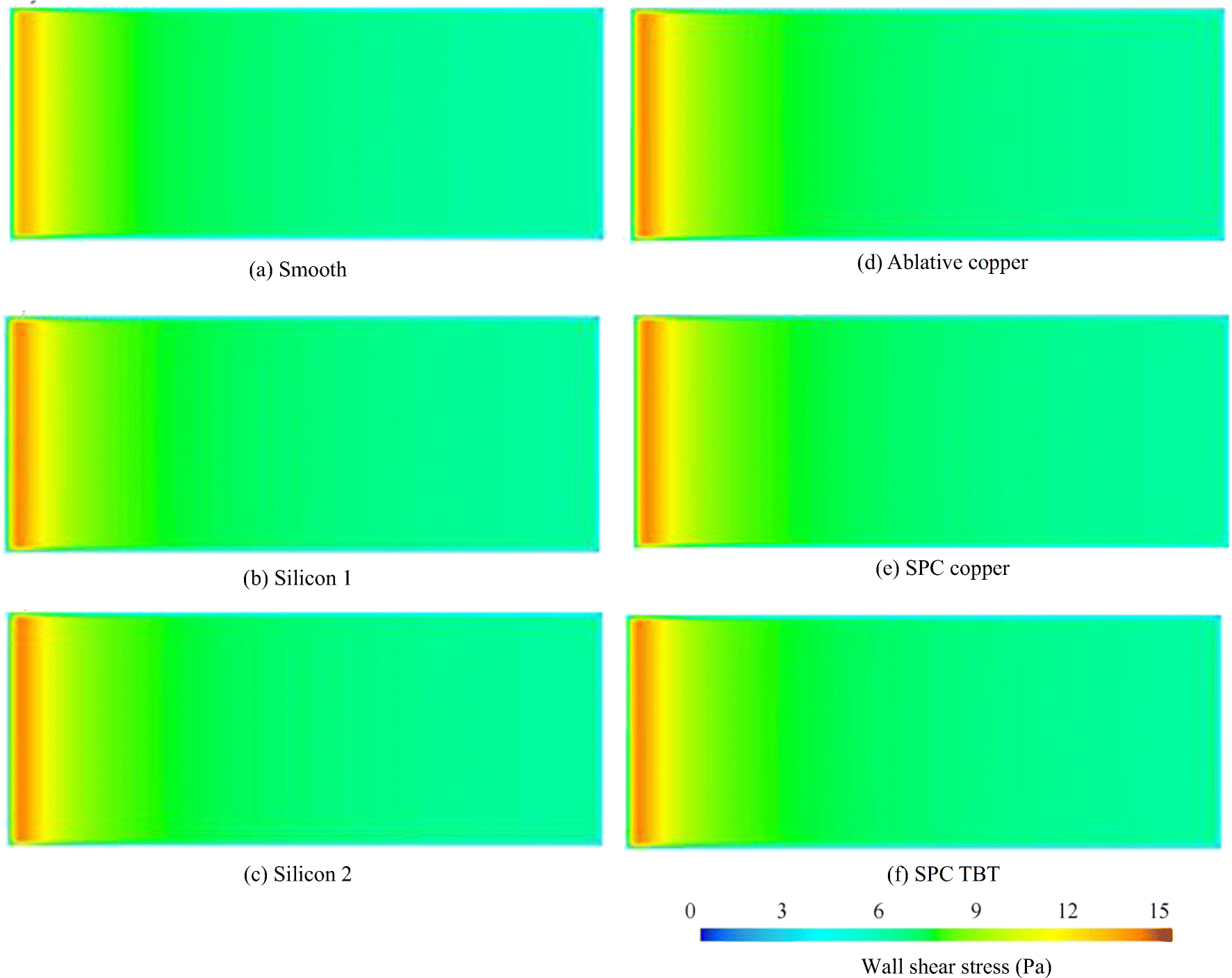 Figure 10 Shear stress distributions on painted surfaces (Re = 2.8 × 10⁶)
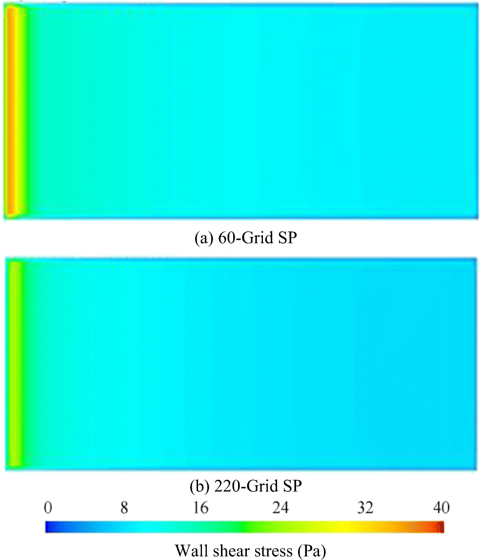 Figure 11 Shear stress distributions on sanded surfaces (Re = 2.8 × 10⁶)
The velocity values at the trailing edge of the plate were compared to examine the surface-related behavior of the normalized mean velocity profile. The downward shift in normalized velocity profiles is shown in Figure 12. Meanwhile, Figure 13 shows the mean velocity and distance relationship over the outer region variables of the turbulent boundary layer. In Figure 11, U+and y+ values were calculated using Eqs. (2)-(4) (Part 2) on the basis of the wall shear stress obtained from the software. In Figure 12, Ue represents the free stream flow velocity, and δ represents the boundary layer thickness assumed as the thickness where flow velocity is equal to 99% of the free stream velocity. The boundary layer thickness was limited as the vertical distance in which the flow velocity in the x direction is equal to 99% of the external flow. Thus, the effect of roughness decreases as it moves away from the wall, and the velocity profiles are consistent with the experimental studies conducted on several rough surfaces (Hama, 1954).
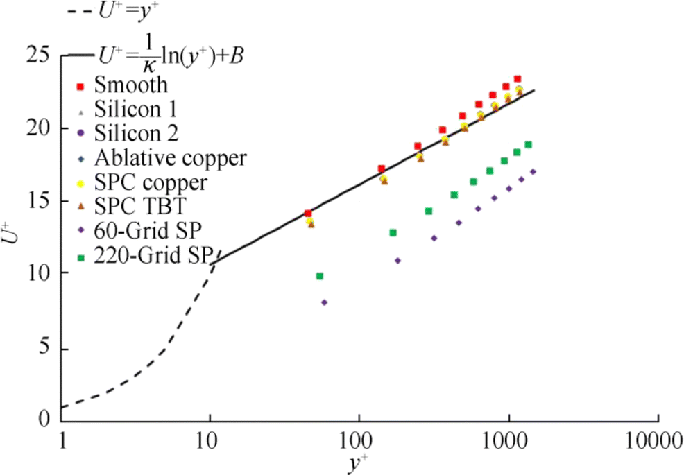 Figure 12 Normalized velocity profiles in the boundary layer (Re = 2.8 × 10⁶)
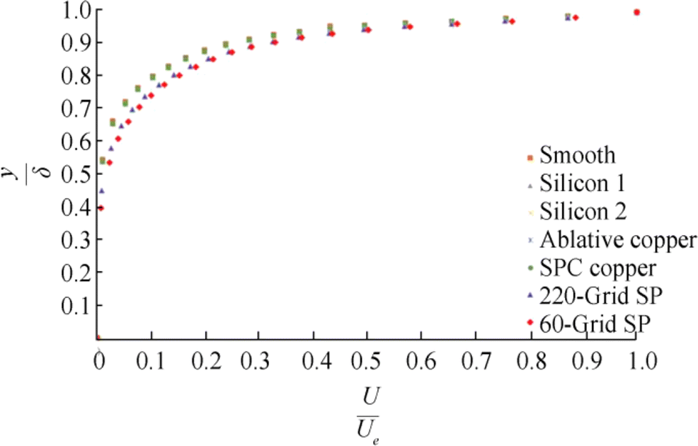 Figure 13 Nondimensional velocity profiles on outer region variables (Re = 2.8 × 10⁶)
7.2 KCS Results
Results obtained with the flat plates indicate that a similar technique can be applied to investigate the flow over other geometries, such those in as ships. The flow around the KCS model was modeled using a similar technique to investigate the effect of roughness on viscous pressure resistance. Unsteady RANS analysis would have been a better way to predict the total resistance of the ship model. However, the purpose of this study is to investigate the viscous resistance components, which are computationally cheap and easy to apply.
The Cf and Cvp values obtained from the analyses performed using the KCS geometry depending on the Froude number are shown in Figures 14 and 15. Cf and Cvp were calculated from Eq. (26), where Rf is the total frictional resistance, R is the total viscous pressure resistance, and S denotes the wetted surface area of the hull. The results indicate that roughness causes an increase in viscous pressure resistance similar to that of frictional resistance.
$$ {C}_f=\frac{R_f}{0.5\rho S{U}^2}\ \mathrm{and}\ {C}_{\mathrm{vp}}=\frac{R_{\mathrm{vp}}}{0.5\rho S{U}^2} $$ (26) 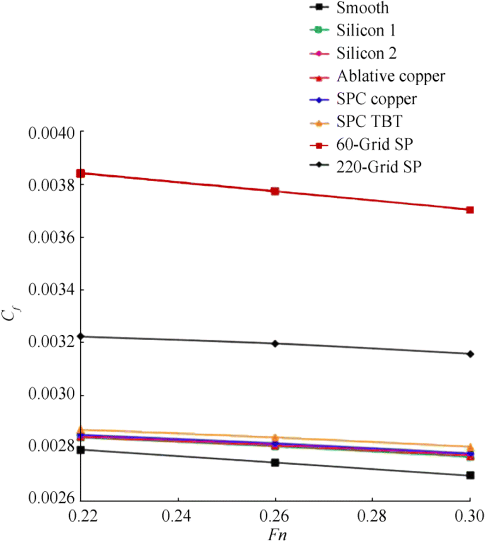 Figure 14 Cf values of the KCS model
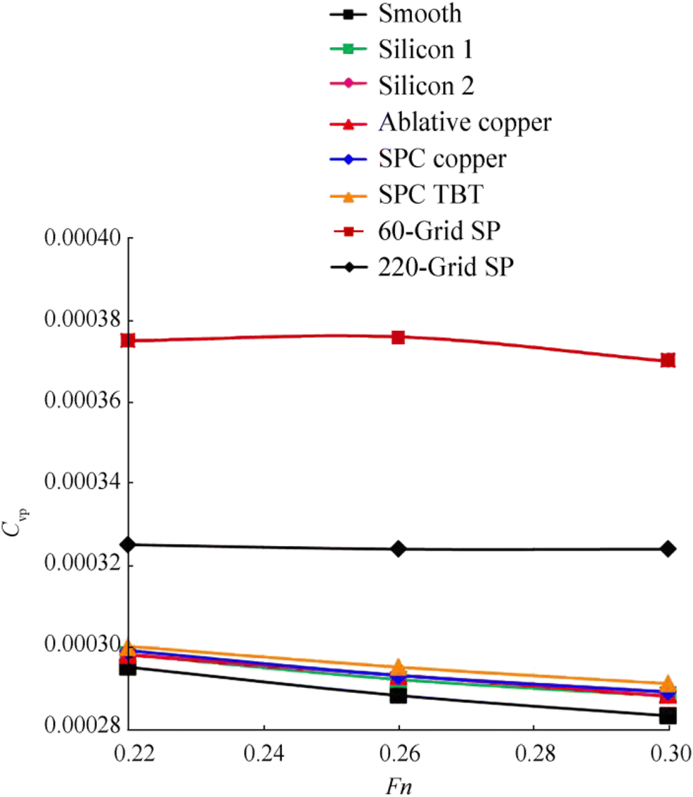 Figure 15 Cvp values of the KCS model
Figure 16 shows the velocity and turbulence kinetic energy distribution on the vessel's midsection plane calculated for Fn = 0.22 of the smooth and 60-grit SP surfaces. The turbulence kinetic energy is increased by surface roughness, whereas the axial velocity values are decreased. Therefore, surface roughness results in the increase in turbulence in the flow and consequently an increase in the shear stress values on the wall and a decrease in the velocity values in the boundary layer. Similar to the Demirel et al. (2017), turbulence kinetic energy and velocity values unexpectedly increase over the plane of symmetry. This increase occurs as a result of the applied symmetry boundary condition.
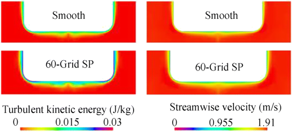 Figure 16 Turbulence kinetic energy and velocity distribution at the midsection
Figures 17 and 18 respectively show the velocity and pressure distributions in the loaded waterline around the smooth surface and the SPC TBT surface at Fn = 0.22. Pressure increases as a result of the decrease in the local velocities at the fore and aft sides of the vessel, and it decreases as a result of the increase in the velocity around the parallel body.
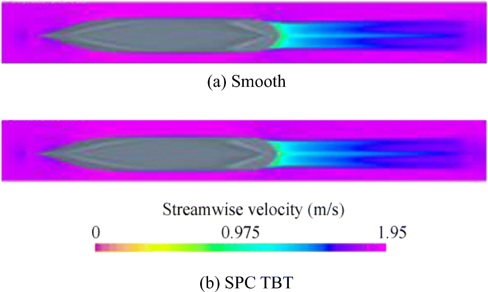 Figure 17 Streamwise velocity distributions at the waterline
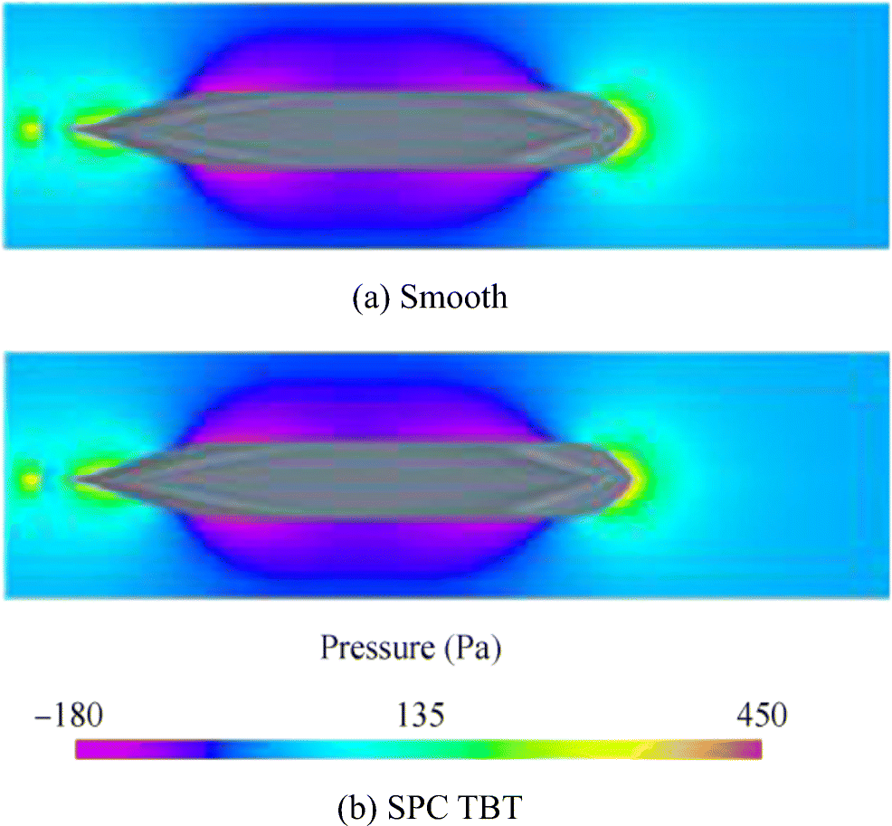 Figure 18 Pressure distributions at the waterline
8 Frictional Resistance at Full Scale
The numerical analysis with the KCS model provides important information on the relationship between surface roughness and viscous pressure resistance. However, these analyses cannot be used to estimate the increase in friction resistance directly at full scale. The reason for this is the change in the physical properties of the problem due to the decrease in the ratio of characteristic height of the roughness and the length of the ship as the length of the ship increases. As the ship length increases, the effect of roughness on the resistance is reduced.
A straightforward way to estimate full-scale resistance characteristics is to conduct RANS analysis on a full-scale vessel rather than a model scale. However, a full-scale RANS analysis requires more computational resources compared with the model scale. In addition, the inner part of the boundary layer is difficult to model because the applied roughness function causes singularities at the average velocities for low y+ values.
In this section, the frictional resistance of the KCS vessel at full scale with service speeds of 20 and 24 knots was predicted, and the full-scale hydrodynamic performance of different antifouling paints was investigated. For this purpose, additional rough surface simulations were performed with flat plates at 20 and 24 kn flow speeds, and roughness functions (∆U+) are calculated using Eq. (25) on the basis of these simulations. Then, the results were extrapolated to ship scale using Granville's similarity law (Granville 1958). A numerical code was developed to calculate full-scale resistance on the basis of plate scale resistance and roughness function (∆U+). The resistance of smooth surfaces was calculated using Schoenherr's (1932) formula. The applied methodology was explained in detail by Demirel et al. (2019) (see also Schultz 2007). Tables 9 and 10 show the Cf coefficients calculated on the plate scale and estimated on the ship scale. The expression ∆Cf represents the increase in frictional resistance due to roughness. At 20 kn, depending on the paint, an increase between 3% and 9% was observed. At 24 kn, the increases were within 4%-8%. Moreover, the ∆Cf values are significantly large at the plate scale.
Table 9 Cf values at plate scale and ship scale (V = 20 kn)Surface Cf (×103) (Plate) ∆Cf% Cf (×103) (Ship) ∆Cf% Smooth 2.675 - 1.357 - Silicon 1 2.915 8.97 1.410 2.96 Silicon 2 2.947 10.2 1.424 6.12 Ablative copper 2.931 9.57 1.417 5.67 SPC copper 2.962 10.7 1.430 6.56 SPC TBT 3.033 13.4 1.462 8.55 Table 10 Cf values at plate scale and ship scale (V = 24 kn)Surface Cf (×103) (Plate) ∆Cf% Cf (×103) (Ship) ∆Cf% Smooth 2.611 - 1.386 - Silicon 1 2.880 10.3 1.427 3.91 Silicon 2 2.914 11.6 1.440 4.94 Ablative copper 2.898 11.0 1.434 4.42 SPC copper 2.931 12.3 1.446 5.38 SPC TBT 3.007 15.2 1.473 7.74 9 Conclusions
In this study, steady RANS equations were solved to examine the turbulent flow properties around the flat plate and KCS model under various surface conditions. The roughness functions were used to model the effects of surface roughness on the mean flow properties within the boundary layer. Grigson-type functions were used on antifouling painted surfaces, and Cebeci- and Bradshaw-type roughness functions were used on sanded surfaces.
The frictional resistance calculated in this study was consistent with the EFD results, except for the surface with the highest roughness height. The relative errors were lower than 3% except for this surface. Therefore, the proposed CFD model can be used to study the hydrodynamic performance of antifouling paints. The most important advantage of the model is that it allows the analysis to be performed with a simple characteristic roughness value based on the surface roughness measurement. Although the determination of the respective roughness for different surfaces requires experimental work, it allows for CFD simulations to be conducted for a wide range of different flow conditions once the appropriate roughness function is determined.
The velocity profile in the boundary layer was examined. The effect of roughness in the outer part of the flow decreases in a similar manner as the previous experimental data. The local shear stress distributions were also examined. The surface roughness showed the highest effect at the flow entrance where the boundary layer is thin.
Analyses with the KCS model showed that the flow behind the body is also significantly affected by the surface condition; thus, the increase in viscous pressure resistance due to roughness is similar to the increase in frictional resistance. However, only a limited range of Reynolds number is covered in this study; thus, inferring that roughness causes an identical increase in frictional and viscous pressure resistance in all scales is impossible. Direct analyses at full scale might be helpful to understand the correlation of these resistance components at full scale. The authors intend to perform further analyses in future studies.
When turbulent kinetic energy and streamwise velocity distributions are examined, an increase in turbulence and boundary layer thickness, leading to a decrease in streamwise velocities, were observed as a result of roughness.
The full-scale frictional resistance calculations indicated that the increase in frictional resistance due to the antifouling paint applications was found to be approximately 3%-9%. The silicone-based foul-release paints result in 3%-4% less resistance when it was first applied.
Furthermore, the proposed method does not cover the free surface effects. Some recent studies reveal that wave resistance is also affected by roughness. The authors intend to cover this point in future studies. Additionally, the use of different roughness functions and the examination of different ship types for some new commercial coatings published in the literature will be investigated.
-
Figure 1 Mean velocity profile in a turbulent boundary layer (Schultz 2004)
Figure 2 Roughness regimes depending on the roughness height (Cal et al. 2009)
Figure 3 Downward shift due to roughness (Demirel et al. 2014)
Figure 4 Dimensions of the plate
Figure 5 Computational domain and boundary conditions for the flat plate
Figure 6 Geometry of KCS
Figure 7 Computational domain and boundary conditions for KCS
Figure 8 Structured grid for flat plate analysis
Figure 9 3D view of the KCS mesh
Figure 10 Shear stress distributions on painted surfaces (Re = 2.8 × 10⁶)
Figure 11 Shear stress distributions on sanded surfaces (Re = 2.8 × 10⁶)
Figure 12 Normalized velocity profiles in the boundary layer (Re = 2.8 × 10⁶)
Figure 13 Nondimensional velocity profiles on outer region variables (Re = 2.8 × 10⁶)
Figure 14 Cf values of the KCS model
Figure 15 Cvp values of the KCS model
Figure 16 Turbulence kinetic energy and velocity distribution at the midsection
Figure 17 Streamwise velocity distributions at the waterline
Figure 18 Pressure distributions at the waterline
Table 1 Roughness statistics of the surfaces (Schultz 2004)
Test surface Ra Rq Rt Silicon 1 12 ± 2 14 ± 2 66 ± 7 Silicon 2 14 ± 2 17 ± 2 85 ± 8 Ablative copper 13 ± 1 16 ± 1 83 ± 6 SPC copper 15 ± 1 18 ± 1 97 ± 10 SPC TBT 20 ± 1 24 ± 2 129 ± 9 60-Grit SP 126 ± 5 160 ± 7 983 ± 89 220-Grit SP 30 ± 2 38 ± 2 275 ± 17 Table 2 General characteristics of KCS
General characteristics Ship scale Model scale Scale - 31.60 Length between perpendiculars (m) 230 7.278 Beam (m) 32.2 1.019 Draught (m) 10.8 0.341 Depth (m) 19 0.601 Block coefficient 0.65 0.650 Wetted surface area (m2) 9424 6.437 Displacement (m3) 52 030 1.648 Table 3 Grid structures and frictional resistance coefficients for flat plate
Cell density Cell number (i × j × k) Cf (CFD) Cf (EFD) RD% Coarse (N3) 199 × 58 × 35 0.003552 0.003605 1.47 Medium (N2) 281 × 82 × 50 0.003548 0.003605 1.58 Fine (N1) 398 × 116 × 70 0.003550 0.003605 1.53 Table 4 GCI calculation results for flat plate
N1, N2, N3 3 231 760, 1 152 100, 403 970 r21, r32 $\sqrt{2} $ ϕ1 0.003550 ϕ2 0.003548 ϕ3 0.003552 p21 0.287 ${\phi}_{21}^{\mathrm{ext}} $ 0.003568 ${\mathrm{GCI}}_{\mathrm{fine}}^{21} $ 0.65% Table 5 Grid Structures and frictional resistance coefficients for KCS
Cell density Cell number Cf (CFD) Cf (ITTC-1957) %RD Coarse (N4) 291 113 0.002667 0.00283 4.03 Medium (N3) 635 417 0.002754 0.00283 0.90 Fine (N2) 1 440 643 0.002748 0.00283 1.11 Finest (N1) 3 268 535 0.002773 0.00283 0.22 Table 6 Grid Structures and frictional resistance coefficients for KCS
N1, N2, N3, N4 3 268 535, 1 440 643, 635 417, 291 113 r21, r32, r43 1.314, 1.313, 1.297 ϕ1 0.002773 ϕ2 0.002748 ϕ3 0.002754 ϕ4 0.002667 p21 6.22 p32 10.63 ${\phi}_{21}^{\mathrm{ext}} $ 0.002779 ${\phi}_{32}^{\mathrm{ext}} $ 0.002748 ${\mathrm{GCI}}_{\mathrm{fine}}^{32} $ 0.01% ${\mathrm{GCI}}_{\mathrm{finest}}^{21} $ 0.25% Table 7 Comparative Cf Values at Re = 2.8 × 10⁶
Surface Cf (×103) (Current Study) Cf (×103) (EFD) Cf (×103) (Demirel et al. 2014) RD% Smooth 3.548 3.605 3.632 1.58 Silicon 1 3.647 3.666 3.715 0.52 Silicon 2 3.662 3.663 3.729 0.03 Ablative copper 3.655 3.701 3.722 1.24 SPC copper 3.669 3.723 3.736 1.45 SPC TBT 3.703 3.783 3.776 2.11 60-grit SP 5.077 6.057 N/A 16.2 220-grit SP 4.317 4.258 N/A 2.40 Table 8 Comparative Cf values at Re = 5.5 × 10⁶
Surface Cf (×103) (Current Study) Cf (×103) (EFD) Cf (×103) (Demirel et al. 2014) RD% Smooth 3.174 3.226 3.185 1.61 Silicon 1 3.315 3.374 3.460 1.75 Silicon 2 3.335 3.426 3.481 2.66 Ablative Copper 3.325 3.401 3.470 2.23 SPC Copper 3.344 3.438 3.491 2.73 SPC TBT 3.392 3.500 3.551 3.09 60-grit SP 4.486 5.954 N/A 24.7 220-grit SP 4.360 4.252 N/A 2.54 Table 9 Cf values at plate scale and ship scale (V = 20 kn)
Surface Cf (×103) (Plate) ∆Cf% Cf (×103) (Ship) ∆Cf% Smooth 2.675 - 1.357 - Silicon 1 2.915 8.97 1.410 2.96 Silicon 2 2.947 10.2 1.424 6.12 Ablative copper 2.931 9.57 1.417 5.67 SPC copper 2.962 10.7 1.430 6.56 SPC TBT 3.033 13.4 1.462 8.55 Table 10 Cf values at plate scale and ship scale (V = 24 kn)
Surface Cf (×103) (Plate) ∆Cf% Cf (×103) (Ship) ∆Cf% Smooth 2.611 - 1.386 - Silicon 1 2.880 10.3 1.427 3.91 Silicon 2 2.914 11.6 1.440 4.94 Ablative copper 2.898 11.0 1.434 4.42 SPC copper 2.931 12.3 1.446 5.38 SPC TBT 3.007 15.2 1.473 7.74 -
Atlar M, Yeginbayeva IA, Turkmen S, Demirel YK, Carchen A, Marino A, Williams D (2018) A rational approach to predicting the effect of fouling control systems on "in-service" ship performance. GMO Journal of Ship and Marine Technology 213: 5-36 Bertram V (2000) Practical ship hydrodynamics. Butterworth-Heinemann Linacre House, Jordan Hill, Oxford Cal RB, Brzek B, Johansson TG, Castillo L (2009) The rough favourable pressure gradient turbulent boundary layer. J Fluid Mech 641: 129-155. https://doi.org/10.1017/S0022112009991352 Candries M, Atlar M, Anderson CD (2001) Foul release systems and drag. Consolidation of Technical Advances in the Protective and Marine Coatings Industry; Proceedings of the PCE 2001 Conference, Antwerp 273-286 CD-ADAPCO (2011) User guide STAR-CCM+. Version 6.06.011 Cebeci T, Bradshaw P (1977) Momentum transfer in boundary layers. Hemisphere Publishing, McGraw-Hill, pp 176-180 Celik IB, Ghia U, Roache PJ, Freitas CJ, Coleman H, Raad PE (2008) Procedure for estimation and reporting of uncertainty due to discretization in CFD applications. J Fluids Eng Trans ASME 130: 078001-1-4. https://doi.org/10.1115/1.2960953 Clauser FH (1954) Turbulent boundary layer in adverse pressure gradients. Journal of the Aeronautical Sciences 21: 91-108. https://doi.org/10.2514/8.2938 Demirel YK (2018) New horizons in marine coatings. GMO Journal of Ship and Marine Technology 213: 37-53 Demirel YK, Khorasanchi M, Turan O, Incecik A, Schultz M (2014) A CFD model for the frictional resistance prediction of antifouling coatings. Ocean Eng 89: 21-31. https://doi.org/10.1016/j.oceaneng.2014.07.017 Demirel YK, Turan O, Incecik A (2017) Predicting the effect of biofouling on ship resistance using CFD. Appl Ocean Res 62: 100-118. https://doi.org/10.1016/j.apor.2016.12.003 Demirel YK, Song S, Atlar M (2019) Practical added resistance diagrams to predict fouling impact on ship performance. Ocean Eng 186: 1-21. https://doi.org/10.1016/j.oceaneng.2019.106112 Farkas A, Degiuli N, Martia I (2018) Towards the prediction of the effect of biofilm on the ship resistance using CFD. Ocean Eng 167: 169-186. https://doi.org/10.1016/j.oceaneng.2018.08.055 Granville PS (1958) The frictional resistance and turbulent boundary layer of rough surfaces. J Ship Res 2: 52-74 https://doi.org/10.5957/jsr.1958.2.4.52 Grigson CWB (1992) Drag losses of new ships caused by hull finish. J Ship Res 36: 182-196 https://doi.org/10.5957/jsr.1992.36.2.182 Haase M, Zurcher K, Davidson G, Binns JR, Thomas G, Bose N, (2016). Novel CFD-based full-scale resistance prediction for large medium-speed catamarans. Ocean Eng, 111(1), 198-208. DOI: https://doi.org/ 10.1016/j.oceaneng.2015.10.018 Haslbeck EG, Bohlander G (1992) Microbial biofilm effects on drag - lab and field. Proceedings of the SNAME Ship Production Symposium. Paper No. 3A-1. Jersey City Hundley L Tate C (1980) Hull-fouling studies and ship powering trial results on seven FF 1052 class ships. D.W. Taylor Naval Ship Research and Development Center Report # DTNSRDC-80/027 111 p IMO (2009) Second IMO (International Maritime Organization) GHG Study, London IMO (2011) Air pollution and energy efficiency, estimated CO2 emissions reduction from introduction of mandatory technical and operational energy efficiency measures for ships. MEPC 63/INF.2 Khor YS, Xiao Q (2011) CFD simulations of the effects of fouling and antifouling. Ocean Eng 38: 1065-1079. https://doi.org/10.1016/j.oceaneng.2011.03.004 Lackenby H (1962) Resistance of ships with special reference to skin friction and hull surface condition. The 34th Thomas Lowe Grey Lecture. Proceedings of the Institute of Mechanical Engineers 176: 981-1014 https://doi.org/10.1243/PIME_PROC_1962_176_077_02 Patankar SV, Spalding DB (1972) A calculation procedure for heat, mass and momentum transfer in three-dimensional parabolic flows. Int J Heat Mass Transf 15: 1787-1806. https://doi.org/10.1016/0017-9310(72)90054-3 Roache PJ (1998) Verification and validation in computational science and engineering. Hermosa Publishers, New Mexico, USA Rushd S, Ashraful I, Sanders RS (2018) CFD methodology to determine the hydrodynamic roughness of a surface with application to viscous oil coatings. J Hydraul Eng 144(2): 04017067. https://doi.org/10.1061/(ASCE)HY.1943-7900.0001369 Schetz JA, Bowersox RDW (2011) Boundary layer analysis, Sec. edn. Prentice-Hall Inc, New Jersey Schlichting H (1979) Boundary Layer Theory, 7th edn. McGraw-Hill, New York Schoenherr KE (1932) Resistance of flat surfaces moving through a fluid. Transactions of the Society of Naval Architects and Marine Engineers 40 Schultz MP (2004) Frictional resistance of antifouling coating systems. ASME J Fluids Eng 126: 1039-1047. https://doi.org/10.1115/1.1845552 Schultz MP (2007) Effects of coating roughness and biofouling on ship resistance and powering. Biofouling 23(5): 331-341. https://doi.org/10.1080/08927010701461974 Shih TH, Liou WW, Shabbir A, Yang Z, Zhu J (1995) A new k-ε eddy viscosity model for high Reynolds number turbulent flows. Comput Fluids 24(3): 227-238. https://doi.org/10.1016/0045-7930(94)00032-T Song S, Demirel YK, Atlar M (2019) An investigation into the effect of biofouling on the ship hydrodynamic characteristics using CFD. Ocean Eng 175: 122-137. https://doi.org/10.1016/j.oceaneng.2019.01.056 Tennekes H, Lumley JL (1972) A first course in turbulence. MIT Press, Cambridge, UK Unal B (2012) Effect of surface roughness on the turbulent boundary layer due to marıne coatings. Istanbul Technical University Institute of Science and Technology, PhD thesis, İstanbul Unal UO (2015) Correlation of frictional drag and roughness length scalefor transitionally and fully rough turbulent boundary layers. Ocean Eng 107: 283-298 https://doi.org/10.1016/j.oceaneng.2015.07.048 UNCTAD (2018) 50 years of review of maritime transport, 1968-2018 - reflecting on the past, exploring the future Wilcox DC (2006) Turbulence modeling for CFD. Third ed, DCW Industries Wolfstein M (1969) The velocity and temperature distribution of one-dimensional flow with turbulence augmentation and pressure gradient. Int J Heat Mass Transf 12:301-318. https://doi.org/10.1016/0017-9310(69)90012-X Yeginbayeva I (2017) An investigation into hydrodynamic performance of marine coatings "inservice" conditions. PhD thesis, Newcastle University, Newcastle