1   Introduction

In the shipbuilding and design industry, the ship dynamics and stability are important design principles that consider the pose and motion characteristics, including capsizing, of ships. Ship motions have six modes or degrees of freedom (i.e., surge, sway, heave, pitch, roll, and yaw). The roll mode has the greatest impact to the capsizing of ships. Most accidents and casualty losses occur due to the lack of understanding the nonlinearity problem of the roll motion system that causes loss of stability. Generally, the prediction methods of roll motion are used as the bases of the equation of motion (EOM) that is employed for determining the response of the roll mode. The EOM consists of the inertia, damping, restoring, and external load F (force or moment) terms, each term performing linear or nonlinear functions. The nonlinear system has more accuracy than the linear system. Hence, the prediction of the nonlinear roll motion system has received attention nowadays. The correction and accuracy of roll prediction depend on the coefficient values or functions of the EOM.

In recent years, many researchers have examined nonlinear characteristics of ship roll motion through experiments and mathematical modeling. For example, Cotton and Spyrou (2001) studied the nonlinear behavior of roll mode and capsizing via experiments. Wassermann et al. (2016) proposed an estimation method of ship roll damping of the decay and harmonic excited roll motion technique for a panamax container ship. Oliva-Remola et al. (2018) proposed an estimation method of damping through internally excited roll motion tests. Haddara and Wu (1993) proposed a parameter identification method of nonlinear roll motion in random seas. Taylan (1999) found the solution of the nonlinear roll model by a generalized asymptotic analysis. Jang et al. (2011b), Kianejad et al. (2019), and Irkal et al. (2019) published articles about the prediction of ship roll damping motion via computational fluid dynamics method. Mancini et al. (2018) published Verification and validation of numerical modeling of DTMB 5415 roll decay. Sathyaseelan et al. (2017) introduced an efficient Legendre wavelet spectral method to the ship roll motion model to investigate nonlinear damping coefficients. Lastly, Jang et al. (2009b) established a novel procedure to identify the functional form of nonlinear restoring forces in a nonlinear oscillatory motion of a conservative system.

Nowadays, the identification of nonlinear system methods has received great attention from many researchers. It has been applied to various branches of science and engineering, particularly in vibration and motion analysis field. The main objective of this method is to obtain a mathematical model based on the requirement of measured data. However, the related studies only considered the nonlinear restoring force or damping force or the simultaneous identification of both, whereas some studies proposed a simultaneous identification method of nonlinear damping and excitation force characteristics (Jang et al., 2011a; Jang, 2013).

Some identification methods for nonlinear restoring force were presented by Masri et al. (1993), Chassiakos and Marsi (1996), and Liang et al. (1997, 2001), who preferred identification based on neural networks. Spina et al. (1996) preferred the nonlinear system identification method from transient data using the Gabor transform based on the application of the Hilbert transform. Moreover, Jang et al. (2009b) proposed a novel method for the nonparametric identification of nonlinear restoring forces in nonlinear vibrations from noisy response data based on the inverse problem. For damping identification only, Iourtchenko and Dimentberg (2002) proposed a procedure for the identification of the damping characteristic from measured stationary responses based on the stochastic averaging method, and Jang et al. (2010a) presented a recovering method for the functional form of nonlinear roll damping with a system identification method using measured response data from a real free-roll decay experiment. Other proponents of the damping identification method are Mohammad et al. (1992), Lazan (1968), Naprstek (1999), and Jang et al. (2010b). The nonlinear identification method can simultaneously identify two force terms of EOM. For instance, Jang (2011) proposed a nonparametric simultaneous identification of the nonlinear damping and restoring characteristics. Jang et al. (2011a) formulated a simultaneous identification method of the nonlinear damping and external harmonic excitation characteristics. Other authors who mentioned the system identification method are Jang et al. (2011b) and Park et al. (2014).

Despite these studies, nobody has examined the simultaneous identification of nonlinear inertia and damping terms based on inverse formalism with measured free decay response data. In fact, the roll motion of the floating body of a single degree of freedom (SDF) in free induction decay consists of acceleration, damping, and restoring moment terms. The nonlinear restoring and damping moments are upon a hull form that functions with the heel angle and angular velocity, respectively. However, the moment due to mass moment of inertia that functions with angular acceleration includes the mass moment of inertia of a floating body and added mass moment of inertia. The added mass moment of inertia is a constant value that is determined by logarithmic decrement (conventional method). Kianejad et al. (2019a, b) discovered the nonlinear behavior of added mass moment of inertia. These discoveries motivated the objective of this study.

The restoring moment can be identified through inclining tests or calculations. The two unknown load functions are added inertia and damping coefficients, and they are presented in this paper based on an inverse problem (Massachusetts Institute of Technology, 2002). The inverse problem seeks to solve an integral equation, which is transformed from nonlinear second-order differential equation and is equivalent to the Volterra-type integral equation of the first kind (Abdul-Majid, 2011). Generally, integral operators are stable, whereas differential operators are unstable. Hence, regularization has a crucial role to solve ill-posed problems, such as numerical instability. In this study, Landweber's regularization method was used to suppress the instability (Qinian, 2011) and the L-curve criteria to determine the optimal solution of the iteration number for the identification.

For the identification example, the proposed procedure was applied to a nonlinear differential equation of the ship roll motion. The numerical experiment reveals the workability of the proposed method for identifying a functional form of both the nonlinear damping and added mass force in a free-roll decay motion.

2   Principles and Theory

To determine a ship roll motion characteristic through the nonparametric identification method, we have to first understand the basics of ship motions and their governing equation (EOM). In reality, a ship simultaneously moves in six directions in a seaway (Volker, 2000), as shown in Figure 1. However, finding all motion characteristics is difficult. Therefore, determining only one direction, namely, SDF, helps reduce the complexity and difficulty. Second, the EOM of SDF is transformed as an integral equation, which has an unknown variable within an integral. Third, the unknown variable is solved via inverse problem formalism and stabilized by Landweber's regularization method. The optimal solution is chosen through the L-curve criterion. Finally, the results of the zero-crossing detection technique of measured data are compared with other solutions to identify the added mass moment of inertia and damping moment and then their nonlinear function formulated.

Figure  1  Modes of ship motion

Download: Full-Size Img

2.1   Ship Rolling and Its Governing Equation

Figure 2 shows an illustration of ship roll motion. It involves restoring moment, damping moment, and moment due to mass moment of inertia that functions with roll angle θ, angular velocity $ \dot{\theta} $, and acceleration $ \ddot{\theta} $, respectively. Normally, a small roll angle of less than 7°–8° (Anthony, 2008) is a linear system. However, in a real seaway, the roll angle should be higher and should have a nonlinear roll motion behavior.

Figure  2  Instantaneous ship roll motion

Download: Full-Size Img

The nonlinear rolling system is governed by a nonlinear EOM that is applied from ordinary differential equation (ODE), which is widely used in the ship motion field.

where $ I\ddot{\theta} $ is the nonlinear moment due to mass moment of inertia function, $ D\left(\dot{\theta}\right) $ is the nonlinear damping moment function, R(θ) is the nonlinear restoring moment function, and M_ext is the external moment function. I is composed of the mass moment of inertia of I_xx and added mass moment of inertia of the ship $ {I}_{xx_a}\left(\ddot{\theta}\right) $. The added mass moment of inertia is functioned with $ \ddot{\theta} $ because it easily identifies and formulates a recovery function.

The function of the restoring moment of a ship can be rewritten in the form $ \overline{\mathrm{GZ}}\left(\theta \right) $ or, as shown in Eq. (3). Accordingly, $ \overline{\mathrm{GZ}}\left(\theta \right) $ is formulated from the $ \overline{\mathrm{GZ}} $ curve in Figure 3 by the curve fitting method with a polynomial function. Moreover, Δ is a ship displacement.

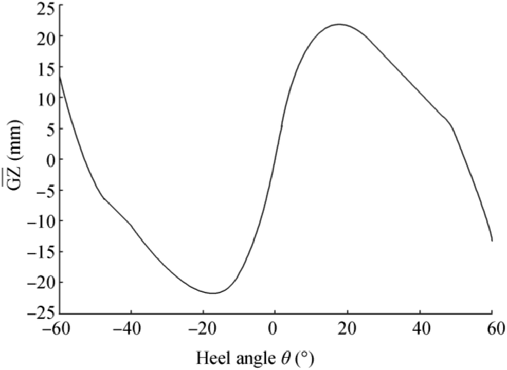Figure  3  Example of a $ \overline{\mathrm{GZ}} $curve versus the heel angle θ

Download: Full-Size Img

By substituting Eqs. (2) and (3) into Eq. (1), the governing equation becomes

This study considers the free-roll decay motion method; thus, M_ext = 0. By rearranging Eq. (4), the governing equation becomes

where kθ is the dummy restoring force, which is added to both sides of Eq. (5), and k is the dummy restoring coefficient value, which is an arbitrary constant value. Let us define

and substitute Eq. (6) into Eq. (5); hence, the governing equation becomes Eq. (7), with the initial values in Eq. (8).

Base on the constant of variation concept, the solutions of Eq. (7) can be written as

and

θ₁ and θ₂ in Eq. (9) are the homogenous solution of Eq. (7), and v₁ and v₂ are the unknown variables. By differentiating Eq. (9), we can obtain

Comparing Eqs. (10) and (11) yields the first condition on v₁ and v₂:

Substituting Eqs. (9) and (10) into Eq. (7) yields the second condition on v₁ and v₂:

Equations (12) and (13) are linear equations for $ {\dot{v}}_1 $ and $ {\dot{v}}_2 $, whose solutions are as follows:

where $ W={\theta}_1{\dot{\theta}}_2-{\dot{\theta}}_1{\theta}_2 $ is called the "Wronskian." The integration and substitution of Eq. (14) into Eq. (7) yield the integral equation form called "the Volterra-type integral equation of the first kind."

where θ₁ and θ₂ are chosen to ensure that they satisfy

where the values of μ and ν are set to be a unit that make the coefficients of first and second terms in the right-hand side of Eq. (15) still equal to initial values as follows: μ = ν = 1 Eq. (8). Thus, the harmonic solutions of Eq. (16) are

where $ \omega =\sqrt{\frac{k}{I_{xx}}} $ is the natural frequency that is a known value.

2.2   Integral Equation

To identify the two unknown quantities $ {I}_{xx}\left(\ddot{\theta}\right) $ and $ D\left(\dot{\theta}\right) $ that are embedded in F(t), Eq. (15) requires the measured system response data, where θ(t) and $ \dot{\theta}(t) $ and its initial conditions follow Eq. (8). For a systematic identification, the method requires a mathematical model that relates the response data to the known variables. Thus, rearranging Eq. (15) to Eq. (18) (Jang et al., 2010a; Jang, 2011) is the formulation for solving F

where

and kernel K is defined as

The left-hand side of Eq. (18) is defined with a new variable, which is a known value from measured data and was called pseudo-displacement by Jang et al. (2011a):

Equation (18) is rewritten as

or can be rewritten in a symbolic form as

where L is the linear integral operator (Jang et al., 2010b):

Equation (18) defines an inverse problem for the simultaneous identification of $ {I}_{xx}\left(\ddot{\theta}\right) $ and $ D\left(\dot{\theta}\right) $. It suffices to prove that its null space is trivial: If θ − αθ₁ − βθ₂ = 0, then F = 0. The proof is the same as that in Jang et al. (2009a) and shows that the equation has a unique solution.

2.3   Solving F by Landweber's Regularization Method

According to the integral equation mentioned above, the unknown F can be calculated under the assumption that η is a continuous function on the time domain, but in fact, the measured data are discrete data: The data are sampled in each time level and have noise. Thus, the noisy data cause the ill-posed problems, the integral equation that makes their solutions lack stability: a small amount of noisy data may amplify a large noisy solution error.

To fix the ill-posed problems, regularization (a stabilization) is used to inhibit the instability. At present, many regularization methods have been used to fix ill-posed problems; the present study has chosen Landweber's regularization method, which is the simplest iterative method. The Moore-Penrose generalized solution (Jang, 2011; Ross, 2014) has to satisfy

where L is an integral operator and L^∗ denotes the adjoint operator of L. When a positive constant λ is multiplied to both sides of Eq. (25), it becomes

and formulated to the iterative method of Landweber's regularization as

The number of iterations and value of λ affect the solution accuracy. The consideration about an optimal number of iterations is decided through the L-curve criterion (Hansen, 2014), which is a stopping rule and is discussed in more detail in "Numerical model example."

2.4   Identifying $ {I}_{xx}\left(\ddot{\theta}\right) $ and $ D\left(\dot{\theta}\right) $ through the Integral Equation

The two unknowns, i.e., a nonlinear added mass moment of inertia $ {I}_{xx}\left(\ddot{\theta}(t)\right) $ and nonlinear damping moment $ D\left(\dot{\theta}(t)\right) $, can be determined through the inverse problems which is determined through Landweber's regularization method. Again, the inverse solution F(t)_inv is equivalent to the right-hand side of Eq. (5):

The pseudo-restoring moment is defined as

The pseudo-restoring moment is the known function that is comprised of the nonlinear restoring and dummy moments. The restoring moment can be identified through a heeling test or calculation, whose function is upon hull geometry. In this paper, the dummy moment is defined with the k value as a unit.

By substituting Eq. (29) into Eq. (28) and rearranging, Eq. (28) becomes

where F_re(t) denotes the remaining moment that is the final moment function; a required function is used for identifying $ {I}_{xx_a}\left(\ddot{\theta}(t)\right)\ddot{\theta}(t) $ and $ D\left(\dot{\theta}(t)\right) $.

The separation between $ {I}_{xx_a}\left(\ddot{\theta}(t)\right)\ddot{\theta}(t) $ and $ D\left(\dot{\theta}(t)\right) $ from the remaining moment requires a zero-crossing time technique, as in Figure 4, where a number of intersection points of the measured data curve of $ \dot{\theta} $ with the time axis are found when $ {t}^d={t}_1^d,{t}_2^d,\dots $ In the same way, there is an intersection of the curve of $ \ddot{\theta} $ with the time axis when $ {t}^m={t}_1^m,{t}_2^m,\dots $:

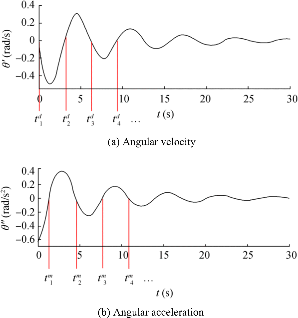Figure  4  Detecting zero-crossing from the measured data of a angular velocity and b angular acceleration

Download: Full-Size Img

The intersection point of both curves holds for the marking point on the remaining moment curve shown in Figure 5. Thus,

and

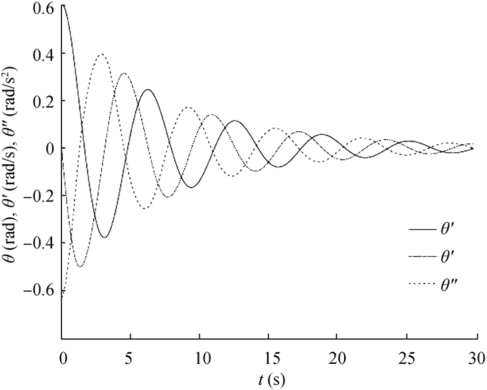Figure  5  Model of the measured data generated by Eq. (41) with the initial condition Eq. (42)

Download: Full-Size Img

From Eq. (31), in the intersection point of $ \dot{\theta} $, the damping moment is zero. Hence, Eq. (33) becomes

Similarly, in the intersection point of $ \ddot{\theta} $, the added moment of inertia is zero. Hence, Eq. (34) becomes

where superscripts m and d denote the mass moment of inertia and damping measured data, respectively, and i denotes the number of the intersection point.

Finally, when collecting all of the intersection points of $ F{\left({t}_i^m\right)}_{\mathrm{re}} $ and $ F{\left({t}_i^d\right)}_{\mathrm{re}} $, we can formulate the functions for each moment function by the appropriate curve fitting method, such as a polynomial function.

3   Numerical Model Example

The proposed scheme demonstrates its workability in identifying the function form of nonlinear added mass moment of inertia and nonlinear damping moment that were carried out through the numerical example.

3.1   Fully Nonlinear EOM

The EOM considered in this study was proposed by Taylan (2000) and is a typical equation of the nonlinear roll motion, which considers that the ship is under the excitation of regular sinusoidal waves:

where ω_e and α_m are the encountered angular frequency and wave slope, respectively. In this study, the proposed scheme is used for free decay testing, so the right-hand side of Eq. (37) is excluded. The three types of nonlinear damping moment functions were classified by Taylan (2000). The nonlinear damping moment function type B1 that is the quadratic equation from Taylan's classification (Taylan, 2000) is chosen for this study:

where D_L and D_N are the linear and nonlinear damping coefficients, respectively. The squared angular velocity term is written as $ \dot \theta \left| {\dot \theta } \right|$ because changing the sign of $ \dot{\theta} $ changes the sign of this term and ensures that damping always opposes the motion.

In general, the cubic and quintic forms of restoring the moment functions are most favorable because they are manipulated easier than higher degree polynomials in the solution procedure (Taylan, 2000). Thus, the restoring moment term is considered by solving Eq. (39).

where C_n, n = 1, 3, 5 are the restoring coefficients of each order. $ {I}_{xx_a} $ in Eq. (37) is normally a constant value, but this study assumed a nonlinear added moment of inertia and its function, following Kianejad et al. (2019). Hence, its magnitude initially increases by increasing the roll angle but quickly declines once the peak value reaches a large roll angle range. However, in this study, the added mass moment of inertia was functioned with angular acceleration, so it was transformed. For simplicity, it was limited to the range before it reaches the peak. Moreover, as the moment of inertia, its function is impossible to be a negative sign when the sign of angular acceleration changes. The expression of the added moment of inertia is as follows:

Thus, Eq. (37) can be rewritten as

with the initial conditions for this experiment given as

For convenience, the values of I_xx and k in Eq. (5) are normalized to units.

For the numerical solution of Eq. (41), the nonlinear ODE was solved by the Runge-Kutta integration scheme with a time step of 0.06 s. The solution and phase diagrams were expressed for D_L = 0.2, D_N = 0.3, C₁ = 0, C₃ = 0.7, C₅ =  − 0.1, and $ {I}_{xx_a}\left(\ddot{\theta}\right)=0.5{\ddot{\theta}}^2 $, as shown in Figures 5 and 6, respectively. This solution was used for the virtual measured data.

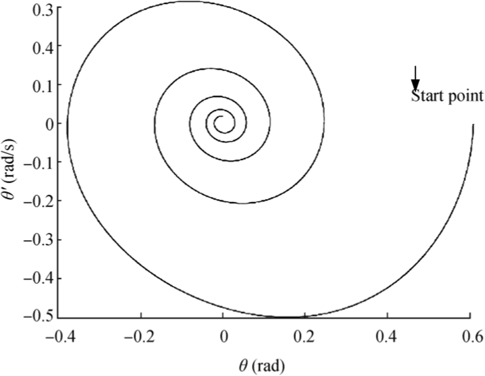Figure  6  Phase diagram corresponding to Figure 5

Download: Full-Size Img

3.2   Noisy Data

The measured data of motion responses have noise. To model the measured data, the noise was generated as follows:

where η^δ is the left-hand side of Eq. (22) and δ is the noise level, where δ  >  0. In this study, δ = 0.001, where ‖·‖₂ denotes the L₂ norm (Filaseta et al., 1992). Thus, we aim to solve the perturbed equation:

3.3   L-Curve Criterion

To solve the perturbed equation, the iteration in Landwerber's regularization method was chosen. The number of iterations plays an important role in the convergence of the solution. The L-curve criterion helps decide the optimal iteration number and results in the best solution.

For selecting the appropriate number of iteration to obtain the optimal solution, the L-curve plots a log-log type of iterated solution norms versus the norm of the corresponding residual, which is represented as follows:

Equation (45) displays the shape of the curve as an "L" shape. The optimum point corresponding to the optimal solution is located at the corner of the curve.

The L-curve is plotted in Figure 7, with δ = 0.001 and λ = 0.001 for Landweber's method in Eq. (27), and obtained the optimal point at j_opt = 10³. The convergence behaviors of the iterative solutions in Figure 8 were observe to match the optimal point from Figure 7 to examine the correct optimal solution. Figure 8b presents the optimal solution obtained from the inverse solution, which was plotted closest to the exact solution and had acceptable stability.

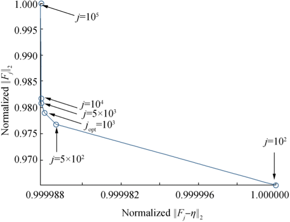Figure  7  Selecting the optimal iteration number from the L-curve

Download: Full-Size Img

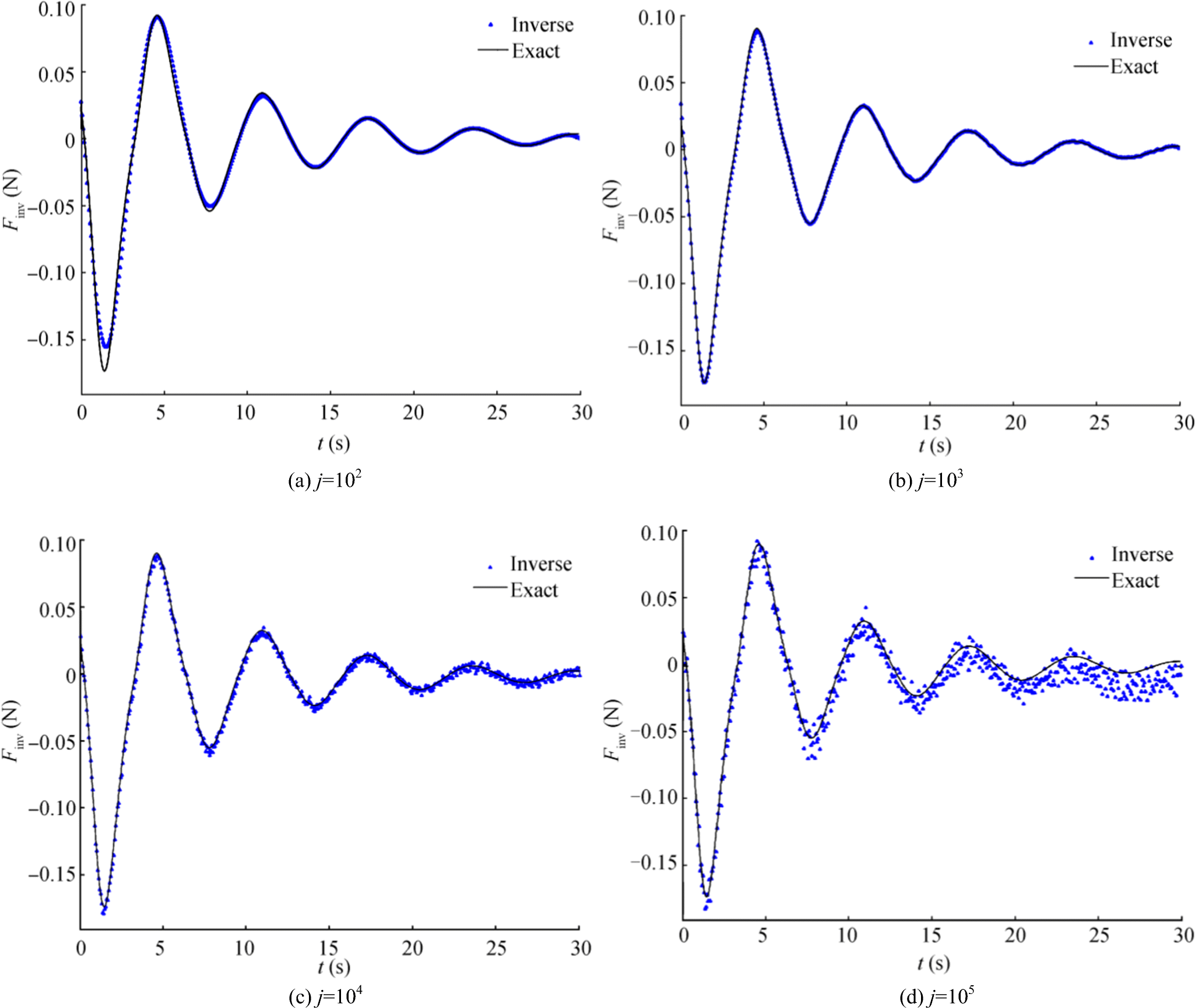Figure  8  Convergence behavior of F_j. The solid line is the exact solution, and the dot point is the regularized solution from Eq. (27). a j = 10². b j = 10³. c j = 10⁴. d j = 10⁵

Download: Full-Size Img

3.4   Recovering $ {{I}}_{{{xx}}_{{a}}}\left(\ddot{{\theta}}\right) $ and $ {D}\left(\overset{.}{{\theta}}\right) $

Following the procedure described in "Identifying $ {I}_{xx}\left(\ddot{\theta}\right) $ and $ D\left(\dot{\theta}\right) $ through the integral equation, " the zero-crossing points of $ \ddot{\theta} $ and $ \dot{\theta} $ were detected and shown at the top of Figure 9 and were held on for comparison with the final inverse solution. The optimal solution from Landweber's regularization method is shown by a dot in the middle part of Figure 9, which also consists of the moments that were explained in Eq. (28). The pseudo-restoring moment F_r in Eq. (29) (known parameter) is plotted with the optimal inverse solution to describe the superposition method for removing F_r from Eq. (28). Thus, the inverse solution F(t)_inv became the final inverse solution F_re that resulted from Eq. (30), which is shown at the bottom of Figure 9. The remaining moments were the final inverse solution that consisted of the moment due to added mass moment of inertia $ {I}_{xx_a}\left(\ddot{\theta}(t)\right)\ddot{\theta}(t) $ and the damping moment $ D\left(\dot{\theta}(t)\right) $. Finally, the separation of these moments was performed through the comparison of detected zero-crossings of $ \ddot{\theta} $ and $ \dot{\theta} $ at the top of Figure 9, which they gave the damping moment and moment due to added mass moment of inertia values at the same time levels, respectively, and were shown at the bottom of Figure 9. The obtained results show that the changing of the positive and negative signs of the moment due to added mass moment of inertia values is similar as that of $ \ddot{\theta} $ at each time level of the $ \dot{\theta} $ zero-crossing. However, the changing of signs of damping moment values is similar as that of $ \dot{\theta} $ at each time level of the $ \ddot{\theta} $ zero-crossing. The signs are written in the anti-symmetric form as follows:

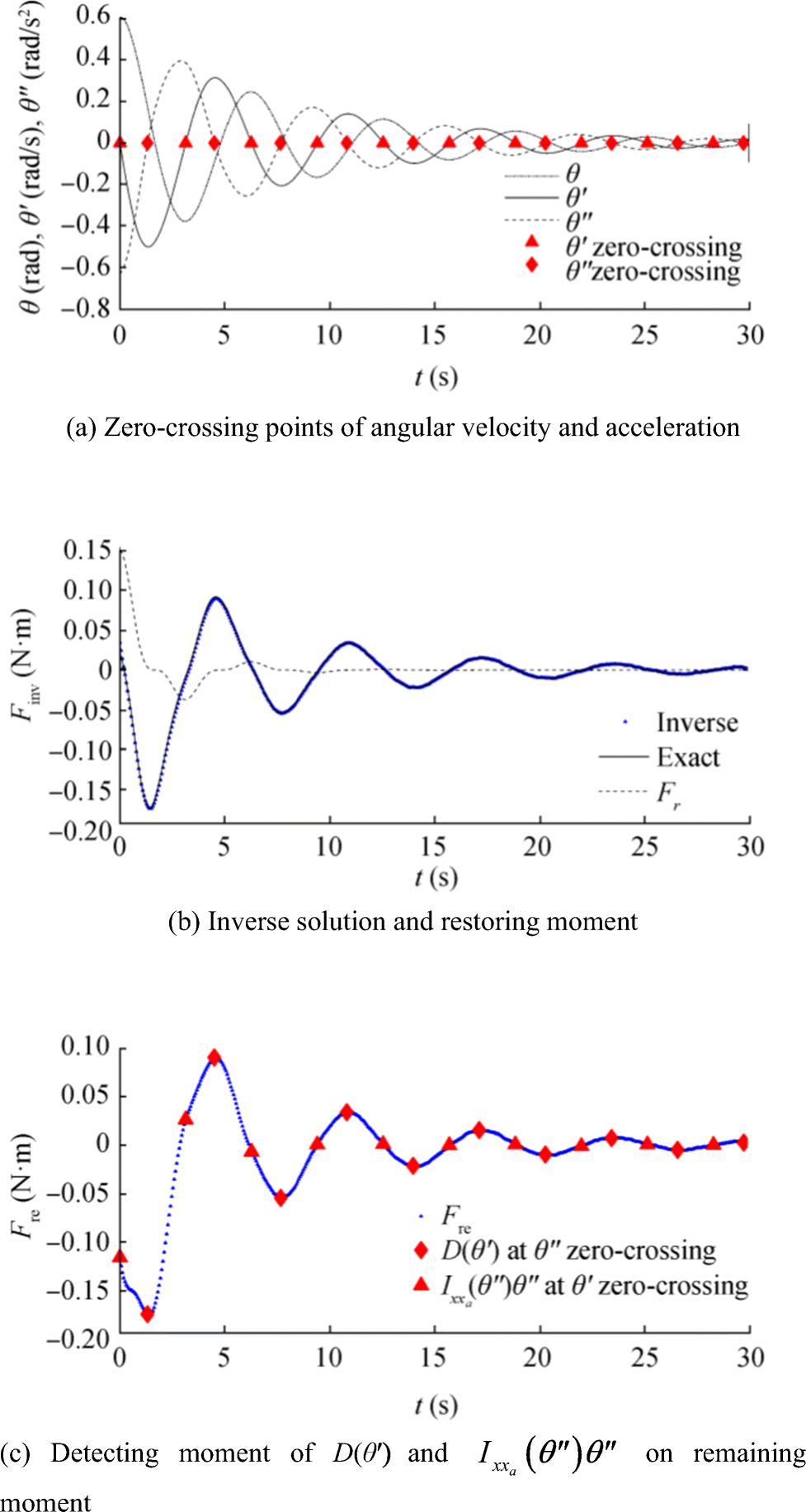Figure  9  Explaining the identifying method of nonlinear moment due to added mass moment of inertia and nonlinear damping moment as follow Eqs. (31)–(36). a Zero-crossing points of angular velocity and acceleration. b Inverse solution and restoring moment. c Detecting moment of D(θ′) and $ {I}_{xx_a}\left(\theta^{{\prime\prime}}\right)\theta^{{\prime\prime} } $ on remaining moment

Download: Full-Size Img

The detected points of the damping and moment due to added mass moment of inertia in the bottom of Figure 9 were re-plotted versus the roll angular velocity and acceleration at the middle and top of Figure 10, respectively. The results of dividing the moment due to added moment of inertia values by the angular accelerations at the same time level became the added mass moment of inertia values that are plotted at the bottom of Figure 10.

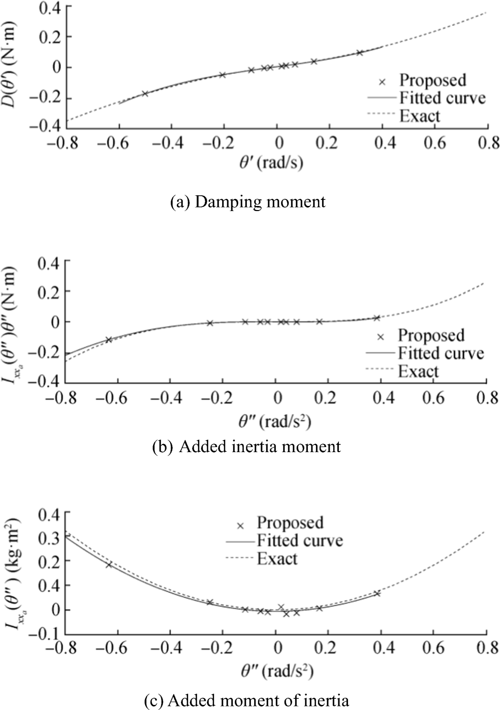Figure  10  Recovered nonlinear moment function: nonlinear damping moment, nonlinear moment due to added mass moment of inertia, and nonlinear added mass moment of inertia. a Damping moment. b Added inertia moment. c Added moment of inertia

Download: Full-Size Img

However, the correct position of a function from data points is still unknown, but hypothetically speaking with experience, a curve from a guessed function must lay on data points as closely as possible. The use of the curve fitting method by a polynomial function is simple and widely used. Thus, in this case, the nonlinear damping moment was fitted by a third-order polynomial function, the nonlinear moment due to added mass moment of inertia was fitted by a fourth-order polynomial function, and the nonlinear added moment of inertia was fitted by a second-order polynomial function. All of the fitted curves were plotted and compared with the exact solution: The top of Figure 10 shows the nonlinear damping moment, the middle of Figure 10 shows the nonlinear moment due to mass moment of inertia, and the bottom of Figure 10 shows the nonlinear added mass moment of inertia. The comparison between the recovered function and exact function gave very good results.

To check and prove the correction and accuracy of the identified moments, Figure 11 shows the plot of the recovered $ \ddot{\theta} $, $ \dot{\theta} $, and θ, which were compared with the exact solution. However, the detected zero-crossing point with one of the initial conditions may not be sufficient to recognize all of the shapes of $ {I}_{xx_a}\left(\ddot{\theta}\right) $ and $ D\left(\dot{\theta}\right) $. For more accuracy, it may need more measured data with different initial conditions.

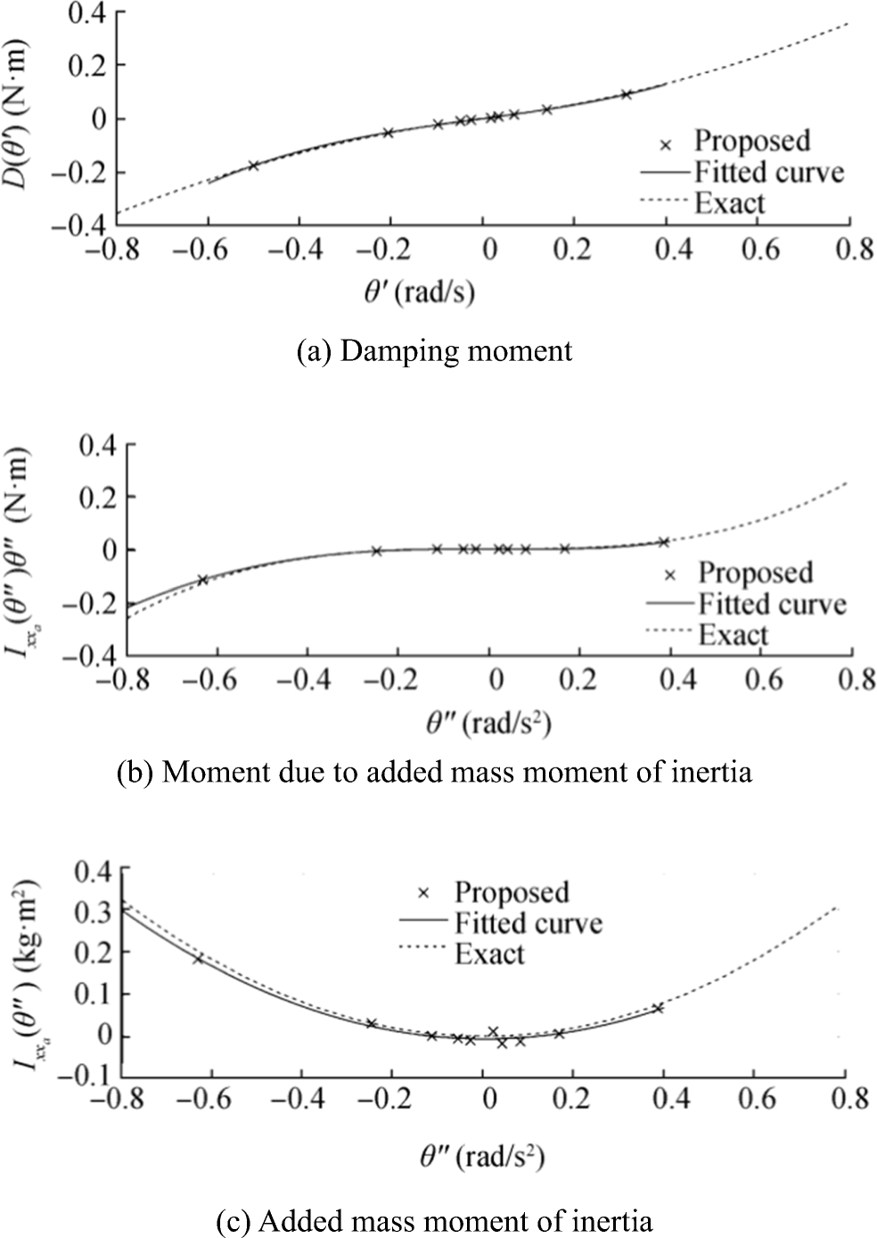Figure  11  Comparison between the exact solution of Eq. (41) and the estimated solution from the recovering nonlinear added mass moment of inertia and nonlinear damping moment function. a Damping moment. b Moment due to added mass moment of inertia. c Added mass moment of inertia

Download: Full-Size Img

4   Conclusions

To determine the nonlinear added mass moment of inertia and damping moment, a nonparametric identification system was used. In this study, the nonparametric identification required an inverse problem that was formulated from the nonlinear EOM. The inverse solution from the numerical method became unstable because of a small amount of noisy data, which can be amplified and lead to unreliable solutions. Accordingly, Landweber's regularization method was used to select the optimal number of iterations through the L-curve criterion. The workability of the proposed procedure is depicted through a numerical example that is fully nonlinear EOM. The results show that the proposed method identified the functional form of the nonlinear added mass moment of inertia and damping moment.