


 , , ,
, , ,
2. International Campus-Mechanical Engineering Group, Amirkabir University of Technology, Tehran 15875-4413, Iran
1 Introduction
Since the Second World War, underwater acoustics has been studied in great detail. Sound propagation through water is the most basic way of communicating in the sea. There are also many other sound sources in the sea such as fish, underwater currents, earthquakes, volcanoes. Therefore, having a clear view of what happens to the generated sounds under the sea surface is an appropriate way of studying natural phenomena in the sea. Sound propagation, noise, and reverberation are three general topics which are considered in order to categorize underwater acoustics(Etter, 2003). Mathematical and physical models are applied in order to study these topics. All these models may contain various boundaries such as sea bed, sea surface, and floating or submerged objects. For instance, in a recent study, Ghadimi et al.(2015a)numerically investigated the effects of a real ocean surface on the incident sound. Also, because of different physical features and factors which are involved in each of these boundaries, they can cause various influences on the incident sound. For instance, at the sea surface, due to the impedance difference between air and water, part of the incident sound is attenuated and the remaining part scattered and transmitted(Godin, 2008). Ghadimi et al.(2015b)numerically studied accuracy of the anomalous transparency of air-water interface theory, which investigates sound transmission at the air-water interface, for a shallow depth source at low frequencies, as proposed by Godin(2008). In addition, environmental conditions at the sea surface such as wind speed, surface roughness, and sub-surface bubbles, are other important factors which can influence the incident sound quality. Therefore, in order to study the sea surface as a boundary in sound propagation, it is important to consider its different characteristics in the suggested mathematical and physical models.
The small perturbation method(SPM)is one of the most important and useful models, and is believed to be an accurate model for studying the effect of the sea surface on incident sound. Because the small perturbation method works better at low frequencies, as mentioned by Thorsos and Jackson(1989), and since publication describing different perturbation methods by Bass(1960) and Marsh(1961), many papers have been published proposing further generalization and applications. Kuo(1985)reported the similarities and differences between these methods in their origin and types of perturbation.
Marsh(1961)developed a general theory of scattering from irregular surfaces, and through an appropriate mathematical description of sea surface, a qualitative account of reverberation was given. Kuo(1988)developed Marsh's perturbation method and proved usefulness of Marsh-Kuo's perturbation method. On the other h and , Bass(1960)divided a velocity potential field into mean and scattered velocity potential fields. His method results in a specular reflection process which approximately satisfies the conservation of energy. Another approach, reported by Brekhovskikh and Lysanov(2003)is quite simple and appealing. Their boundary condition is only perturbed to the first order in surface roughness h. Applying their approach, it is easily possible to obtain unknown mean and scattered velocity potentials. Both Marsh(1961) and Brekhovskikh and Lysanov(2003)went beyond the perturbation approximation in order to obtain a closed-form solution for the scattering loss.
However, Kuo(1994)by utilizing joint surface roughness and volumetric perturbation scattering theory, characterized bubbly ocean surface reverberation. Then, he showed the backscattering strength predictions to be consistent with observed reverberation phenomena, such as critical wind speeds, excess levels due to volumetric scattering, and saturation. Ghadimi et al.(2015c)developed an approach based on the optimized Helmholtz-Kirchhoff-Fresnel method and verified the accuracy of Kuo's approach in modeling surface scattering of sound in various environmental conditions.
In a recent study, Ghadimi et al.(2015d)studied sound scattering in the Persian Gulf based on empirical relations. However, the main aim of this paper is to provide an approach to theoretically study sound scattering in the Persian Gulf based on the prominent Kuo small perturbation method. Therefore, this paper is organized as follows: First, in Section 2, crucial relations of SPM theory developed by Kuo(1994)are presented briefly. In Section 3, wind speed and wave height in the Persian Gulf region are discussed extensively, according to different databases. In Section 4, SPM theory is first verified by CST-7 test results, as reported by Ogden and Erskine(1994a; 1994b). Nicholas et al.(1998)proposed an empirical relationship, based on CST-7 results, to calculate scattering strength from the sea surface. Their relationship, at low frequencies and wind speeds, depends on SPM(Etter, 2003). Therefore, real CST-7 data, with uncertainties to 5 dB, is utilized in order to show SPM's accuracy. Consequently, by applying Kuo's approach(Kuo, 1994)in this paper, sound scattering from a rough bubbly sea surface in the Persian Gulf region is studied and predictions for sound scattering are presented. Accordingly, SPM theory based on Kuo's approach(Kuo, 1994)is discussed and , based on the presented environmental conditions in the Persian Gulf, sound scattering from the sea surface is examined. Finally, Section 5 summarizes the current findings and offers conclusions. The produced results may help investigators in various areas, including sea surface wave studies, sound propagation, and noise pollution, under various environmental conditions in the Persian Gulf.
2 Small perturbation methodDue to its complications, a real sea surface has great influence on incident sound. Hence, in order to obtain accurate solutions for the scattering coefficients, it is necessary to include significant factors in the proposed physical and mathematical models. For example, wind speed, which causes surface roughness and generates sub-surface bubbles through breaking waves, is believed to be an important factor in sound scattering phenomena from such rough bubbly water surfaces. As mentioned, Kuo's approach(Kuo, 1994)in SPM is based on Marsh's perturbation theory(Marsh, 1961). He further developed Marsh's approach and exp and ed his theory to more realistic sea surface conditions. He considered a rough bubbly sea surface as a region in which volumetric and roughness scattering occur(Fig. 1). Both the rough interface and bubbly surface layer are assumed to be effectively infinite in horizontal extent, and solutions to all r and om scattering fields are obtained. A planar wave velocity potential is considered to enter the wind-generated bubbly layer shown in Fig. 1 and it is defined as
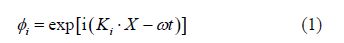
where Ki is the incident sound wave number, X is the position vector, is angular frequency and t is time. Two different sequences of events can be assumed for the entry wave.

|
| Fig. 1 Schematic of rough bubbly region at the sea surface |
The first sequence starts from volumetric scattering of the incident wave(Fig. 2). The up-going volumetrically scattered waves then surface and volumetrically scatter again. The scattered field generated by alternating repeated scattering events will eventually become negligible.

|
| Fig. 2 Down-going and up-coming volumetrically scattered waves |
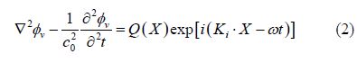
The second sequence starts from a rough surface scattered wave velocity potential, (Fig. 3). The surface scattered waves will be volumetrically scattered, followed by similar alternating scattering processes as the first sequence until the scattered waves become negligible. The total reflected field is the combination of all the down-going waves described above. According to Batchelor's relation(Batchelor, 1956), the volumetric scattered field in the first sequence of events satisfies the relation:

|
| Fig. 3 Incident wave is surface scattered as |
where
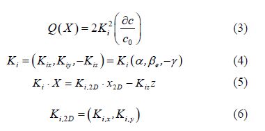
Here, and are respectively cosine of the wave number vector with respect to x, y, and z axes, and is the fractional acoustic velocity fluctuation where c0 is the sound speed in water. The scattering phenomenon will continue until waves lose all their energy. Hence, it is possible to neglect high order scattered waves in the first sequence of events.
The second sequence of events starts from the surface scattering of the incident wave . This phenomenon is shown in Fig. 3. The surface-scattered wave will then be volumetrically scattered to produce both a down-going wave and an up-going wave . The up-going wave will be volumetrically and surface scattered until its complete attenuation.
Fractional acoustic velocity fluctuation can be expressed in terms of many different but interrelated physical quantities that are denoted by a general physical variable in the following equation:
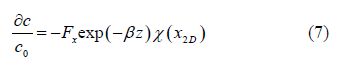
where is a constant related to depth, z is the bubbly water depth, 1 500 m/s is the sound speed in water, and is a r and om physical variable representing a particular selected physical property. Based on the chosen, takes a different expression. Numbers of bubbles per unit volume N, acoustics scattering cross section per unit volume Mv, roughness element height, fraction of white cap coverage W, are various physical parameters which can be considered as in Eq.(7).
For instance, if is chosen to be roughness element height, the following expression can be defined for :
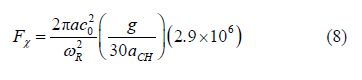
where a is bubble radius, c0 is the sound speed in water, 0.018 5 is Charnock's constant, is bubble resonant circular acoustic frequency, is the resonant frequency, and g is gravity acceleration.
Kuo(1994), through some calculations, defined scattering coefficient s from the sea surface based on, , and which are respectively wave spectra of surface roughness, r and om physical parameter, and cross correlation of .Hence, Kuo(1994)defined scattering coefficient s from the sea surface through the following relation:
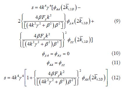
In Eq.(9), and are defined as
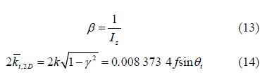
where, f is sound frequency, k wave number, grazing angle, and cosine of incident sound grazing angle. Wu(1992)defined the following relations for according to wind speed
0.4 m, 7 m/s(15)
0.4+0.12(U‒7) m 7 m/s(16)
Therefore, it is possible to calculate the sea surface scattering coefficient by applying Eq.(9). In the next section, the Persian Gulf's environmental conditions are presented in order to examine sound surface scattering in this region.
3 Geographical and climate condition of the Persian GulfThe Persian Gulf is located in the middle east south of Iran(Fig. 4). It is a semi-enclosed sea that is connected east through the Strait of Hormuz and the Gulf of Oman to the Indian Ocean. Its area is approximately km2; its western end is marked by the major river delta of the Shatt al-Arab, which carries the waters of Euphrates and the Tigris. Its length is 989 km with Iran along most of the northern coast and Saudi Arabia alongthe southern coast. It is about 56 km wide at its narrowest, the Strait of Hormuz. The water is overall very shallow, with a maximum depth of 90 m and an average depth of 10 m(Zhang, 2011). The Persian Gulf and its coastal area are the world's largest sources of crude oil, and related industries dominate this region. Large gas finds have also been made, with Qatar and Iran sharing a giant field across their median territorial line.

|
| Fig. 4 The Persian Gulf geographical location(Location of Arzanah station is indicated) |
The Persian Gulf has relatively warm weather, and seasonal north-west winds are the most powerful, mostly blowing in summer and winter. From November to March, seasonal winter winds blow from west to east. This phenomenon creates a cold weather front which causes seasonal north-west winter winds to blow in December, January, and February. Seasonal summer winds, which usually blow from the beginning of June to the middle of July, are weaker than the seasonal winter winds. They occur due to low pressure thermal conditions in the Indian Ocean and the Oman Sea.
Annual and seasonal wind rose plots reported by Arzanah station in the 5 year period, 2003 to 2007, are shown in Fig. 5 and Fig. 6. Also, Table 1 presents hourly wind speeds as well as annual and seasonal gust information as reported by Arzanah station.

|
| Fig. 5 Annual wind rose plot reported by Arzanah station during 2003 to 2007(Golshani, 2010) |

|
| Fig. 6 Seasonal wind rose plots reported by Arzanah station during 2003 to 2007(Golshani, 2010) |
| Season | Hourly wind speed | Gusty wind speed | ||||
| Max. | Mean | Variance | Max. | Mean | Variance | |
| April and May | 16.0 | 4.68 | 2.66 | 19 | 6.64 | 3.12 |
| June to middle of July(summer winds) | 17.5 | 4.71 | 2.45 | 21 | 6.66 | 2.87 |
| Middle of July to August | 12.5 | 3.77 | 2.01 | 15 | 5.61 | 2.47 |
| September and October | 12.5 | 3.55 | 1.82 | 15 | 5.30 | 2.27 |
| November and March(winter winds) | 17.5 | 5.16 | 2.83 | 20 | 7.17 | 3.21 |
| December to February(winter winds) | 15.0 | 5.63 | 2.89 | 17.5 | 7.75 | 3.30 |
| Annual | 17.5 | 4.67 | 2.64 | 21 | 6.64 | 3.08 |
There are other data bases besides Arzanah station. Numerical models such as NCEP/NCAR(NOAA, 2009), ERA40(ECMWF, 2009), and PERGOS(Ocean weather, 2009)provide data which can be accessed freely on their websites. These numerical methods, and their approach towards obtaining environmental variables, are defined in their websites in more detail. The QuikSCAT satellite(PODAAC, 2007)also presents its data on its website. Different features of these data bases are provided in Table 2. Table 3 provides the wind speed information from each data base. Wind rose plots resulting from the numerical and satellite data are also shown in Fig. 7.
| Data base | *Data type | Period | Time step/h | Geographical coordinates | |
| Wind | Wave | ||||
| Arzanah station | × | × | 1/1/2003 to present | 3, 6, 12(mostly 3) | 52.5667 East 24.7833 North |
| Numerical model NCEP/NCAR | × | - | 1/1/1948 to 12/31/2007(60 years) | 6 | 52.5 East 25.7139 North |
| Numerical model ERA40 | × | × | 9/1/1957 to 8/31/2002(46 years) | 6 | 52.5 East 25 North |
| Numerical model PERGOS | × | × | 1/1/1983 to 12/31/2002(20 years) | 1 | 52.5625 East 24.5 North |
| QuikSCAT satellite(NASA) | × | - | 7/1/1999 to present | At least 12 | 52.625 East 25.625 North |
| * Available information are shown by ‘×', unavailable information are shown by ‘-'. | |||||
| Database | Max. | Mean | Variance |
| Arzanah station | 17.50 | 4.68 | 2.64 |
| Numerical model(NCEP/NCAR) | 16.72 | 4.29 | 2.38 |
| Numerical model(ERA40) | 15.03 | 4.52 | 2.38 |
| Numerical model(PERGOS) | 15.99 | 4.35 | 2.01 |
| QuikSCAT satellite(NASA) | 28.94 | 5.98 | 2.73 |

|
| Fig. 7 Wind rose plots(Golshani, 2010) |
According to Table 3, the reported wind speed by QuikSCAT satellite is larger than that reported by other data. Golshani and Taebi(2008)concluded that the reported data by QuikSCAT are valid in a wind speed range of 5-15 m/s. Furthermore, since the time step of QuikSCAT satellite data base is also larger than those reported by other data bases, some geographical and climate phenomena with shorter time steps cannot be reported. This is particularly evident in Table 2 in which the time steps for many data bases(ranging from 3 to 6 hours)is less than that for QUIKSCAT data base(which is 12 hours). Also, based on Table 4, it is seen that QUIKSCAT does not report wave height information. Therefore, one can conclude that the QUIKSCAT data base is not suitable for the aim of the current paper.
However, since Arzanah station, ERA40, and PERGOS data bases have shorter time steps and provide wave height information, they are deemed appropriate for being used by the SPM method.
As seen in Table 4, the maximum and mean values for rms wave heights in ERA40 are less than the two other databases. Wave rose plots for the databases listed in Table 4 are shown in Fig. 8. Since wind speeds and wave heights in the Persian Gulf are availabe from different databases, the necessary information for applying the SPM method are available. Therefore, it is possible to study surface scattering of generated sound in the Persian Gulf.
| Database | Max. | Mean | Variance |
| Arzanah station | 3.3 | 0.63 | 0.42 |
| ERA40 | 2.89 | 0.41 | 0.4 |
| PERGOS | 3.1 | 0.57 | 0.37 |

|
| Fig. 8 Rms of wave heights(Golshani, 2010) |
There are different theoretical and empirical methods to calculate the period of wind-generated waves. Among them, Parvaresh et al.(2005)used the auto correlation function(ACF)with real required parameters, from the Ports and Shipping Organization of Iran, to calculate dominant wave periods in the Persian Gulf. Auto correlation coefficients were determined based on different time lags, shown in Fig. 9.

|
| Fig. 9 Dominant wave periods with 1 hour time lag(Parvaresh et al., 2005) |
Wind speed as well as sea surface wave height and period are required in order to apply SPM theory. Based on the environmental conditions described here, sound scattering from the Persian Gulf's surface will be discussed in the following section.
4 Surface scattering by SPM in the Persian GulfIn the previous sections, SPM and environmental conditions in the Persian Gulf were discussed. Also, it was mentioned that SPM is an appropriate approach by which it is feasible to examine sound scattering from a bubbly rough sea surface.
Since in the current paper, sound scattering from the Persian Gulf's surface is of interest, the next step is to analyze its acoustic characteristics, based on the environmental conditions provided in section three.
It is a common practice to examine surface acoustic roughness to determine whether a surface is acoustically rough. A measure of the acoustic roughness of the sea surface is provided by the Rayleigh parameter R through the following relationship:
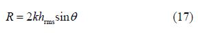
where is the acoustic wave number, is the acoustic wave length. When, the sea surface is considered to be acoustically smooth; when, the surface is acoustically rough(Etter, 2003). In Eq.(17), is the parameter which is related to the environmental condition whereas k and are related to the sound source. Fig. 10 shows the Persian Gulf's surface acoustical roughness, based on the mean and max. rms wave heights in Table 4 at three frequencies 100, 500 and 1 000 Hz. As evident in Fig. 10(a), as sound frequency increases at mean surface wave heights, acoustical roughness increases. Also, as shown in Fig. 10(b), at max. rms wave heights, the sea surface can be considered acoustically rough. When the sea surface is rough, the vertical motion of the surface modulates the amplitude of the incident wave and superposes its own spectrum, as upper and lower sideb and s, on the spectrum of the incident sound(Etter, 2003). Since SPM considers surface roughness effects, it is an appropriate model to study sound scattering from a rough surface such the Persian Gulf.

|
| Fig. 10 The Persian Gulf's surface acoustical roughness according to reported sea surface wave heights by Arzanah, ERA40 and PERGOS databases |
The term in Eq.(12), which is the wave spectrum, modulates the surface roughness effects on the incident sound. In order to determine this factor Pierson-Moskwitz's wave spectrum(Pierson Jr and Moskowitz, 1964), which is defined as Eq.(18), is applied.
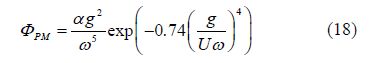
where 0.008 1, (rad/s)is the circular frequency of the sea surface, g is the gravity acceleration and U(m/s)is the wind speed. If Eqs.(13), (14) and (18)are substituted in Eq.(12), scattering coefficient from the sea surface can be obtained through the following expression:
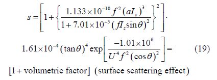
As evident in equation(19), resulted scattering coefficient s from SPM consists of the two components surface roughness and volumetric scatterings.
Fig. 11 depicts surface wave spectra vs. circular frequency based on reported wind speeds by Arzanah, PERGOS, and ERA40 databases. It can be seen that as the wind speed increases wave spectra increase. Also, wave spectra approximately reach peaks at circular frequencies 2 rad/s and 0.6 rad/s at mean and max.reported wind speeds, respectively. However, based on Fig. 9, which depicts dominant wave periods of the irregular surface waves of the Persian Gulf, its circular frequencies based on mean and max. wave periods are 12.3 rad/s and 44.9 rad/s, respectively. At these circular frequencies, the sea surface wave spectra are in the order of 10−5. But since irregular sea surface waves consist of many regular surface waves with various amplitudes and wavelengths, their acoustical behavior differs from their total wave period. In fact, incident acoustic waves can occupy sea surface wave periods which are in their frequency range(Kuo, 1994). Therefore, the sea surface wave spectrum of the corresponding acoustic frequency should be considered for acoustic computations. Consequently, Kuo(1994)suggests considering the incident sound frequency as the input of the Pierson-Moskwitz relation to obtain . As evident in Fig. 11, for a broad frequency range, when frequency decreases, surface waves' spectra increase. Consequently, as will be discussed, surface scattering strengths decrease.

|
| Fig. 11 Surface wave spectrabased on Arzanah, PERGOS and ERA40 databases |
As discussed in Section 2, in addition to surface roughness scattering, which depends on the surface wave spectrum, volumetric scattering can play an important role in the total scattering strength. In the SPM method, dominant subsurface bubble radius is the volumetric parameter in the computations. The radius of wind generated bubbles usually varies in the range of 10 μm to 100 μm. Hence, the dominant bubble radius a can be considered to have an approximate mean value of 60 μm(Medwin and Clay, 1998).
In order to demonstrate the effectiveness of the SPM method, its results are compared against the results of critical sea tests 7(CST-7)provided by Ogden and Erskine, 1994a; 1994b. These tests were conducted for various source frequencies, grazing angles, and wind speeds, with uncertainties in the calculations of about to 5 dB. Such uncertainty should be assigned to all the results of CST-7(Ogden and Erskine, 1994a; 1994b). Through these tests, they concluded that there are three different regimes involved in sound scattering from the sea surface. In the first regime, surface roughness scattering is the dominant mechanism at the sea surface. This mechanism plays an important role at low frequencies and low windspeeds. In the second regime, subsurface bubble population is the dominant mechanism. As frequency and wind speed increase, the second regime becomes dominant. In the third regime, which is called transitional regime between the other two regimes, both surface and roughness mechanisms are involved in sound scattering from the sea surface(Ogden and Erskine, 1994a; 1994b). Since SPM has both volumetric and surface roughness components, the SPM results can be verified by the reported scattering strengths' data of CST-7.
As mentioned in section two, the SPM method, through parameter, is dependent on wind speed. Wu(1992)defined a critical wind speed as the dominant mechanism for different combinations of wind speed and frequency. Below the critical wind speed, surface roughness scattering is dominant, and above, volumetric scattering is dominant(Kuo, 1994). Therefore, based on the defined critical wind speed at each frequency, it is possible to determine the dominant regime. Fig. 12 depicts SPM results at wind speeds 2.57 m/s and 15.43 m/s; with frequencies 50 Hz and 100 Hz. According to Ogden and Erskine(1994a; 1994b), at these wind speeds scattering strength is dominated by roughness scattering rather than volumetric scattering. So the first regime is dominant. Consequently, the volumetric scattering component of SPM is not included in the total scattering results since it is zero. Fig. 13 represents the volumetric and roughness components of the scattering strength at 1 000 Hz and at wind speeds 2.57 m/s and 15.43 m/s. Unlike the considered cases in Fig. 12, here the volumetric component of surface scattering affects its total value, especially at low grazing angles. As evident in Fig. 13, the volumetric component increases the total scattering strength results in the second and the third regimes.

|
| Fig. 12 Volumetric, roughness and total scattering strengths at wind speeds of 2.57 m/s and 15.43 m/s; and at frequencies of 50 Hz and 100 Hz |

|
| Fig. 13 Volumetric, roughness and total scattering strengths at wind speeds of 2.57 m/s and 15.43 m/s at frequency of 1 000 Hz |
Fig. 14 shows the results of SPM and CST-7 tests vs. grazing angle at wind speed 5 m/s and 100 Hz and 1 000 Hz. Based on Ogden and Erskine's conclusion(Ogden and Erskine, 1994a; 1994b), at this wind speed all the frequencies are located in the first regime's region. Therefore, surface roughness scattering is the dominant mechanism. As evident in Fig. 14, the SPM results have a good agreement with the CST-7 tests. In Fig. 15, wind speed is increased to 15 m/s at the same frequencies of Fig. 14. At frequency 100 Hz and wind speed 15 m/s, the first regime is dominant. But at frequency 1 000 Hz and wind speed 15 m/s, the second mechanism is dominant. Therefore, a subsurface bubble population is the dominant mechanism at frequency 1 000 Hz. Compared to the SPM results for the first regime, in the second regime scattering results diverge from the CST-7 results as the grazing angle increases. Considering uncertainties in parameter defined by Wu(1992), Kuo(1994)mentions that SPM results are acceptable. Also, Thorsos and Jackson(1989)mention that SPM is more accurate at low frequencies and low wind speeds. However, as evident in Fig. 14 and Fig. 15, by increasing the frequency at constant wind speed, scattering strength increases. As depicted in Fig. 11, this seems to be reasonable due to the fact that an increase in frequency decreases surface spectrum and consequently increases scattering strength(Kuo, 1994).

|
| Fig. 14 Results of SPM and CST7 test at wind speed of 2.57 m/s(CST-7 by Ogden and Erskine(1994b)) |

|
| Fig. 15 Results of SPM and CST-7 test(Ogden and Erskine, 1994b)at wind speed of 15.43 m/s |
In Fig. 16 and Fig. 17, grazing angles are considered constant being 10° and 30°, respectively. In these figures, scattering strengths are shown vs. wind speeds at three different frequencies. Fig. 16 presents the scattering strengths at frequencies 50 Hz, 200 Hz, and 1 000 Hz. Here, at 50 Hz, the first regime is dominant at all wind speeds, based on Ogden and Erskine, and at frequency 200 Hz, the first and third regimes are involved. However, at 1 000 Hz, all three regimes are involved as wind speed increases. As observed in Fig. 16, the SPM results have a good agreement with CST-7. This figure also indicates that frequency increase causes a general increase in scattering strength. Since frequency and wind speed range, which determine the dominant regimes in Fig. 17 are similar to Fig. 16, the regime behaviors at various frequencies as wind speed increase, are alike. Here also, the results of SPM and CST-7 display good agreement.

|
| Fig. 16 Results of SPM vs. CST-7 test(Ogden and Erskine, 1994b)at grazing angle of 10° |

|
| Fig. 17 Results of SPM vs. CST-7 test(Ogden and Erskine, 1994b)at grazing angle of 30° |
Fig. 18 to Fig. 20 present the results for the SPM method for sound scattering from the sea surface in the Persian Gulf based on different databases. Each figure represents the mean and maximum values of wind speed for an individual database.

|
| Fig. 18 Scattering strength(dB)by SPM method based on Arzanah Station |

|
| Fig. 19 Scattering strength(dB)according to ERA40 model |

|
| Fig. 20 Scattering strength(dB)according to PERGOS model |
As evident in Fig. 14 through Fig. 17, the SPM method provides reasonably good results compared with real open field data for the Gulf of Alaska, and therefore can be considered as an appropriate method for investigating sound scattering in the different open field of the Persian Gulf, where there is actually no experimental data available for sound scattering.
Fig. 18 through Fig. 20 provide scattering strength results in the Persian Gulf based on the environmental conditions presented in Section 3. Required input data for SPM is depicted in the caption of each figure. Fig. 18, which presents the SPM results based on Arzanah station data, shows scattering strength vs. sound frequency for the mean and maximum wind speeds. In Fig. 18(a), since the considered wind speed is less than the critical wind speed at different frequencies, the first regime is dominant. Therefore, scattering strength results are controlled by the surface roughness scattering mechanism. In Fig. 18(b), based on the considered wind speed of 17.5 m/s, which is above critical wind speed in all grazing angles and above 200 Hz, the second and the third regimes are dominant. As mentioned, in these regimes volumetric scattering affects the total scattering strength results. Here, the general trend of CST-7 results, scattering strengths in the first regime are less than in the third regime, can be seen. Furthermore, SPM is based on four different environmental and source parameters: wind speed U, rms of wave height, frequency f, and grazing angle θ. Comparison of the mean and maximum wind speed values shows that scattering strength generally increases as wind speed increases. Also, as mentioned earlier, frequency increase results in increase of the scattering strength.
Fig. 19 presents the scattering strength calculated by SPM based on the ERA40 model. Here, the dominant regimes are similar to Fig. 18, so the scattering strength trends are the same. Fig. 20 shows the calculated scattering strength based on the PERGOS database.
5 ConclusionsThe SPM has been developed over past decades to become a more effective and accurate model. This development has occurred due to the increasing number of effective variables involved in sound scattering from the sea surface. In this paper, Kuo's SPM method is applied in order to predict surface scattering strengths in the Persian Gulf region. Therefore environmental conditions in the Persian Gulf are surveyed. Subsequently, five different numerical and station databases are presented and used to study the wind speed and wave height in this region. These databases are compared and three of them are found to be the most appropriate and so selected to be used in the SPM method. Accordingly, data provided by Arzanah station, ERA40, and PERGOS databases are utilized by the SPM method to predict surface scattering. Calculated results indicate scattering strength increases as frequency, grazing angle, and wind speed increase. Plots of scattering strength vs. grazing angle by the SPM method for different frequencies and wind speeds are presented and compared against the results of critical sea tests 7(CST-7). These comparisons show favorable agreement that is indicative of the fact that Kuo's SPM method can accurately model and predict sound scattering from the sea surface in various environmental conditions such as different wind speeds, surface wave heights, and wave periods. These results might help acousticians study various acoustics related phenomena in the Persian Gulf environment, including the effects of propagated sound from oil exploration and production activities on marine life, calibration of instruments, such as acoustic Doppler current profiler(ADCP)which study sea surface waves.
| Bass FG (1960). Boundary conditions for the average electromagnetic field on a surface with random irregularities and with impedance fluctuations. Izv. Vuzov, Radio Fizika, 3, 72-78. |
| Batchelor GK (1956). Wave scattering due to turbulence. In: Sherman FS. Symposium on Naval Hydrodynamics. National Academy of Sciences-National Research Council, Washington, DC, USA, 430. |
| Brekhovskikh LM, Lysanov YP (2003). Fundamentals of ocean acoustics. Springer, New York, USA. |
| ECMWF (2009). ECMWF products. European centre for medium-range weather forecasts. Available from http://old.ecmwf.int/products [Available from Aug. 27, 2010]. |
| Etter PC (2003). Underwater acoustic modeling and simulation. 3rd ed., Spon Press, New York, USA. |
| Ghadimi P, Bolghasi A, Feizi Chekab MA (2015a). Acoustic simulation of scattering sound from a more realistic sea surface: Consideration of two practical underwater sound sources. Journal of the Brazilian Society of Mechanical Sciences and Engineering. DOI: 10.1007/s40430-014-0285-1 |
| Ghadimi P, Bolghasi A, Feizi Chekab MA (2015b). Low frequency sound scattering from rough bubbly ocean surface: small perturbation theory based on the reformed Helmholtz-Kirchhoff-Fresnel method. Journal of Low Frequency Noise, Vibration and Active Control, 34(1), 49-72. DOI: 10.1260/0263-0923.34.1.49 |
| Ghadimi P, Bolghasi A, Feizi Chekab MA (2015c). Sea surface effects on sound scattering in the Persian Gulf region based on empirical relations. Journal of Marine Science and Application, 14(2), 113-125. DOI: 10.1007/s11804-015-1306-x |
| Ghadimi P, Bolghasi A, Feizi Chekab MA, Zamanian R (2015d). Numerical investigation of transmission of low frequency sound through a smooth air-water interface. Journal of Marine Science and Application, 14(3), 334-342. DOI: 10.1007/s11804-015-1315-9 |
| Godin OA (2008). Low-frequency sound transmission through a gas-liquid interface. The Journal of the Acoustical Society of America, 123(4), 1866-1879. DOI: 10.1121/1.2874631 |
| Golshani A (2010). Wave properties in Persian Gulf according to SWAN model. Journal of Marine Engineering, 6(12), 73-87. (In Persian) |
| Golshani AA, Taebi S (2008). Evaluation of wind vectors observed by QuikSCAT/seawinds using synoptic and atmospheric models data in Iranian adjacent seas. Journal of Marine Engineering, 4(8), 47-63.(In Persian) |
| Kuo EYT (1985). The origin of different acoustic perturbation scattering concepts of rough random surfaces. Naval Underwater Syst. Ctr., New London, USA, Tech. Memo. 861166. |
| Kuo EYT (1988). Sea surface scattering and propagation loss: Review, update, and new predictions. IEEE Journal of Oceanic Engineering, 13(4), 229-234. DOI: 10.1109/48.9235 |
| Kuo EYT (1994). The perturbation characterization of reverberation from a wind-generated bubbly ocean surface, I: Theory and a comparison of backscattering strength predictions with data. IEEE Journal of Oceanic Engineering, 19(3), 368-381. DOI: 10.1109/48.312913 |
| Marsh HW (1961). Exact solution of wave scattering by irregular surfaces. The Journal of the Acoustical Society of America, 33(3), 330-333. DOI: 10.1121/1.1908654 |
| Medwin H, Clay CS (1998). Fundamentals of acoustical oceanography. 2nd ed., Academic Press, Boston, USA. |
| Nicholas M, Ogden PM, Erskine FT (1998). Improved empirical descriptions for acoustic surface backscatter in the ocean. IEEE Journal of Oceanic Engineering, 23(2), 81-95. DOI: 10.1109/48.664088 |
| NOAA (2009). PSD climate and weather data. Earth System Research Laboratory, NOAA. Available from http://www.cdc.noaa.gov/data/ [Available from Feb. 20 2015]. |
| Ocean weather (2009). Met ocean studies. Ocean Weather Inc. Available from http://www.oceanweather.com/metocean/ [Available from Apr. 5, 2001]. |
| Ogden PM, Erskine FT (1994a). Surface and volume scattering measurements using broadband explosive charges in the critical sea test 7 experiment. The Journal of the Acoustical Society of America, 96(5), 2908-2920. DOI: 10.1121/1.411300 |
| Ogden PM, Erskine FT (1994b). Surface scattering measurements using broadband explosive charges in the critical sea test experiment. The Journal of the Acoustical Society of America, 95(2), 746-761. DOI: 10.1121/1.408385 |
| Parvaresh A, Hassanzadeh S, Bordbar MH (2005). Statistical analysis of wave parameters in the north coast of the Persian Gulf. Annales Geophysicae, 23(6), 2031-2038. DOI: 10.5194/angeo-23-2031-2005 |
| Pierson Jr WJ, Moskowitz L (1964). A proposed spectral form for fully developed wind seas based on the similarity theory of S. A. Kitaigorodskii. Journal of Geophysical Research, 69(24), 5181-5190. DOI: 10.1029/JZ069i024p05181 |
| PODAAC (2007). QuikSCAT. Jet Propulsion Laboratory, California Institute of Technology. Available from http://podaac.jpl.nasa.gov/quikscat [Available from Feb. 20, 2015]. |
| Thorsos EI, Jackson DR (1989). The validity of the perturbation approximation for rough surface scattering using a Gaussian roughness spectrum. The Journal of Acoustical Society America, 86(1), 261-277. DOI: 10.1121/1.398342 |
| Wu J (1992). Individual characteristics of whitecaps and volumetric description of bubbles. IEEE Journal of Oceanic Engineering, 17(1), 150-158. DOI: 10.1109/48.126963 |
| Zhang Z (2011). Spectral decomposition using S-transform for hydrocarbon detection and filtering. Texas A & M University, College Station, USA. |