


 , ,
, ,
2. Port and Maritime Organization, Tehran 6316-15875, Iran
1 Introduction
Having information about wave spectrum is among the most important requirements in different maritime engineering activities e.g. coastal engineering, port engineering and offshore engineering(Wang, 2014; Tanaka and Yokoyama, 2004). There are different well-known wave spectra in which each are useful under certain circumstances. These are models extracted based on field data at specified regions and wisely or blindly extended overseas. However, such an approach of implementing a st and ard spectrum model is practical. A comprehensive review of such st and ard models is also available(Chakrabarti, 2005).
Since 1953 and the introduction of first two-parameter spectral model by Newman(Chakrabarti, 2005), there have been great achievements in its development(Young, 1998; Pierson Jr and Moskowitz, 1964; Hasselmann et al., 1973). This has resulted in today’s common st and ard models recommended by rules and regulations. Among them are PM model(Pierson Jr and Moskowitz, 1964), JONSWAP model(Hasselmann et al., 1973) and more recently, ITTC model(ITTC, 2002). It should be noted that all such models have their own pros and cones when used for other seas. So, calibration has always been an issue for researchers.
It is now evident that for a fully arisen sea condition the PM spectrum could be utilized to describe spectral characteristics(Pierson Jr and Moskowitz, 1964; Wen, 2011). However, for a growing sea state the JONSWAP spectrum could be implemented(Hasselmann et al., 1973)even though they still suffer from the lack of accuracy. Ochi and Hubble(1976)ascertained that all wave spectra such as JONSWAP spectrum are good approximations for different conditions if the parameters are tuned well enough as illustrated by other reasearchers(Young, 1998; Zahibo et al, 2008; Eldeberky, 2011). Such efforts to modify JONSWAP spectrum was continued by Kumar and Kumar(2008). Also, Manzano-Agugliaro et al.(2011)tried to extract a spectral model considering recorded data at the Strait of Gibraltar. Finally, Akers and Nicholls(2012 ; 2014)studied the spectrum of periodic traveling gravity waves.
While such st and ard spectra have been used throughout these years, published precious measured data at the Strait of Hormuz together with the importance of this region resulted in conducting present research to assess capability of such models. Therefore, after a short introduction of measurement stations the spectral model has been briefly investigated by their wave rose in section two. The storm software, which is a product of Nortek, is used to process data series in accordance with Nortek acoustic wave and current profiler(AWAC)as the measurement tool. The mentioned software uses the fast Fourier transform(FFT)method to extract field spectrum. Consequently, performance of the aforementioned st and ard spectra is evaluated in section three. Finally, distinguished spectral models have been calibrated based on statistical measures. The study evidently showed the importance of such valuations especially when there are enough amounts of recorded data.
2 MeasurementIn 2008, a comprehensive field measurement program has been carried out in the Strait of Hormuz in order to monitor and model the Iranian coasts by the Iranian Ports and Maritime Organization. In this paper, wave measurement data were collected by AWAC at four different stations and are presented in Table 1 and Fig. 1. It should be noted that UTM coordinates are one of the universal grid systems based on a family of 120 transverse Mercator map projections(two for each UTM zone, with one for each N/S hemisphere).
| Station No. | Depth/m | Measurement time interval | Measurement point coordination(UTM) | |||
| Start | End | X | Y | Zone | ||
| 1 | 25 | 2009/12/09 | 2010/08/07 | 708 098 | 2 972 528 | 39 |
| 2 | 25 | 2009/10/09 | 2010/12/10 | 250 901 | 2 905 642 | 40 |
| 3 | 25 | 2009/06/10 | 2011/27/06 | 430 486 | 2 966 586 | 40 |
| 4 | 25 | 2010/04/09 | 2011/17/05 | 575 653 | 2 832 497 | 40 |

|
| Fig. 1 Locations of measurement stations |
Before analyzing the data, a series of pre-processing st and ardizing operations should be taken to eliminate unphysical data. There are many types of error in recording wave data in which Gap and Spike could be pointed out as the most common errors. Also, errors due to the device operation such as vibrations(vessels collision to buoy)can cause the error. Common errors in recording data have been described as follows(Casas Prat, 2009):
· Spike: In this case, the height of wave changes irrationally and does not follow its pre and post tendency.
· Gap: In this case, no data have been recorded in a time interval and therefore the values of this interval are shown as zero or irrational numbers.
Among the data measured, two different groups of data could be observed including data without error, data with low error and data with high error. The data with low error analogous is shown in Fig. 2 and such parts should be replaced by interpolations(Kuik et al., 1988). For high error parts analogous as shown in Fig. 3, such intervals should be excluded. All in all, high errors resulted in eliminating two percent of measured data.

|
| Fig. 2 Spike with low error at station 1 |

|
| Fig. 3 Spike with high error at station 2 |
In Figs. 4 to 7, the wave rose at all stations are presented. It is obvious that the dominant direction is different at such stations. In order to assess the performance of selected st and ard spectral models, extreme events at dominant directions have been extracted for each station, assuming an appropriate threshold of ${{H}_{m0}}\ge {{1}^{m}}$. Table 2 shows the range of wave height changes, the range of related peak period changes and the number of hurricanes detected at each station.

|
| Fig. 4 Wave rose at station 1 |

|
| Fig. 5 Wave rose at station 2 |

|
| Fig. 6 Wave rose at station 3 |

|
| Fig. 7 Wave rose at station 4 |
| Direction of extreme event | Range of significant wave height | Range of peak wave period | Number of events detected ( Hm0 ≧1m ) |
| West- Northwest | 1-2.91 | 2.19-8.49 | 190 |
| West | 1-2.63 | 2.22-9.27 | 115 |
| South- Southwest | 1-2.24 | 2.15-9.77 | 340 |
| Southeast | 1-1.95 | 3.04-7.26 | 56 |
The data presented in Fig. 8 shows that peak period Tp varies between $\text{2}\sqrt{{{H}_{m\text{0}}}}$ and ${\text{8}}\sqrt {{H_{m{\text{0}}}}}$ thatis different from those values suggested by International Ship Structures Congress(ISSC)(Mazaheri and Ghaderi, 2011; Parvaresh et al., 2005)as well as what found by Kumar and Kumar(2008)for other ocean waves.

|
| Fig. 8 The relationship between peak wave period and significant wave height at different directions |
After extracting dominant events at each station, comparisons could be made between observed spectra and those presented by st and ard models at this step.
Actually, different spectra could be used to answer this main question in ocean engineering that what would be an appropriate presentation of ocean waves. Perhaps the simplest is that proposed by PM in 1964(Pierson Jr. and Moskowitz, 1964; Lucas at al., 2011)under fully developed sea condition. PM and ITTC later introduced at the ITTC(ITTC, 2002)models that follow a general form as Eq.(1)
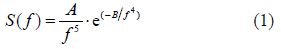
In which for Pieson Moskowitz wave spectrum $A = 0.0081{g^2}{(2{\text{\pi }})^{ - 4}}$ and $B = 0.0324{g^2}/[{(2{\text{\pi }})^4}H_s^2]$, also for ITTC wave spectrum $A = 0.312H_s^2f_p^{ - 4}$ and $B = 1.25f_p^{ - 4}$. Here, f is frequency in Hz, g is the acceleration of gravity in m/s2, fp is peak frequency in Hz and Hs is significant wave height in m.
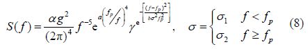
During assessment of field data, Hasselmann et al.(1973)found that wave is never fully developed and always continues to develop. Therefore, they added an extra factor to that of PM in order to improve the fit to their measurements. However, for the JONSWAP model the most widely used spectral model is presented as below:
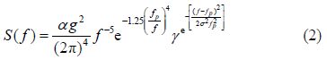
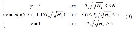
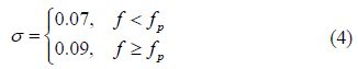
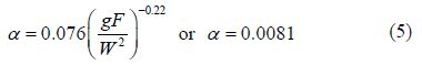
They also facilitate the use of this model in which γ could be a constant between 1 and 7. γ=3.3 and α=0.008 1 are the most recommended values as used in this study for the st and ard version of JONSWAP spectrum. There are also some reports in which researchers have tried to calibrate such parameters(Ochi and Hubble, 1976; Tolman et al., 2005; Kumar and Kumar, 2008; Belibassakis et al., 2014; Akhmediev et al., 2015; Srisuwan and Work, 2013).
In the following, the st and ard JONSWAP, PM and ITTC spectral models are investigated. For this statistical assessment, Δfp and ΔA have been used as the difference between observed and modeled peak frequency as well as spectrum integral, respectively. Besides, two other quantities(R2 and NError)have been implemented. The aforementioned quantities are presented as below:
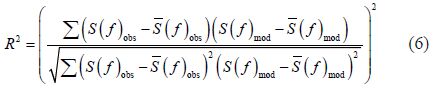
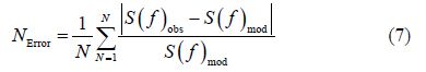
R2 and NError are criterions to check trend similarity and value conformity. Suffixes "obs" and "mod" st and for observed and modeled spectra, respectively. Such parameters have been selected in a way to report most important statistical aspects of conformity between observation and model.
According to these measures, performance of such examinations comparing observed and st and ard spectra is reported in Table 3 for all stations. It should be noted that, fp entered directly to JONSWAP and ITTC. So, Δfp=0 is not a great achievement and we will get back to this issue later in model calibration. However, ITTC results are more promising than two other spectra. JONSWAP is weaker in modeling the environment, but having fp as one of its inputs pushes one to go further.
Fig. 9 compares an observed spectrum with JONSWAP, PM and ITTC models at a typical event. It should be noted that the reported values are just the average ones. Consequently, they might be larger in some cases than others, as is the case for Fig. 9.

|
| Fig. 9 Comparison of an observed spectrum with selected models for a typical West-Northwest wave of Hs=1.30 m and Tp=5.27 s |
Considering Table 3 results together with the very first aim of this study, it is now time to go a step further taking some effort to calibrate st and ard spectra. For this reason, JONSWAP and ITTC models have been considered. The PM model is excluded from the list due to its lack of sensing fp as mentioned earlier as well as its imperfect statistical assessment results especially when compared with those of ITTC model.
| Extreme event direction | Spectral model | R2 | NError/% | Δ fp/Hz | ΔA/m2 |
| West-Northwest | JONSWAP | 0.80 | 28 | 0 | 0.270 |
| PM | 0.60 | 21 | 0.07 | 0.002 | |
| ITTC | 0.83 | 14 | 0 | 0.003 | |
| West | JONSWAP | 0.75 | 30 | 0 | 0.290 |
| PM | 0.50 | 22 | 0.04 | 0.002 | |
| ITTC | 0.82 | 9 | 0 | 0.002 | |
| South-Southwest | JONSWAP | 0.81 | 27 | 0 | 0.250 |
| PM | 0.53 | 24 | 0.06 | 0 | |
| ITTC | 0.90 | 10 | 0 | 0.002 | |
| Southeast | JONSWAP | 0.76 | 29 | 0 | 0.300 |
| PM | 0.50 | 26 | 0.05 | 0.002 | |
| ITTC | 0.85 | 10 | 0 | 0.003 |
So, to achieve a higher accuracy, predefined constant coefficients of such models have been changed in order to achieve more concordance of observed and modeled spectra at the Strait of Hormuz.There are absolutely some papers dealing with st and ard methodologies in calibration of JONSWAP spectrums(Yilman, 2007; Violante-Carvalho et al., 2002). But, generalized reduced gradient(GRG)nonlinear algorithm(Abadie, 1978)as a general tool in practice is used to introduce higher R2 while keeping NError, Δfp and ΔA at minimum values. In should be noted that such a combination has been found the best in a trial and error procedure. The conformity of maximum values of observed and calibrated spectra is also checked together with other four statistical measures to select between different combinations ahead to force in the calibration procedure.
4.1 Calibration of JONSWAP model
For the JONSWAP model, it could be parameterized by introducing five potential parameters α, a, b, σ1 and σ2 for calibration, as below:
To increase accuracy, GRG nonlinear algorithm results in coefficients presented in Table 4 for each station and /or direction. The result is called direction sensitive calibration version or simply calibrated version. It is apparent that NError experiences great lessening up to 50% at South-Southwest event direction as well as R2 with encouraging increase up 30% at west event direction. However, a pattern of improvement is obvious at all other stations. It is interesting that σ1 and σ2 faces no change when compared with their original value.
| Model | Extreme event direction | α | γ | σ1 | σ2 | a | b | NError | R2 | Δ A/m2 | Δfp/Hz |
| St and ard JONSWAP model | West-Northwest | 8.1×10⁻³ | 3.30 | 0.07 | 0.09 | −1.25 | 2 | 0.28 | 0.80 | 0.27 | 0 |
| West | 8.1×10⁻³ | 3.30 | 0.07 | 0.09 | −1.25 | 2 | 0.30 | 0.75 | 0.29 | 0 | |
| South-Southwest | 8.1×10⁻³ | 3.30 | 0.07 | 0.09 | −1.25 | 2 | 0.27 | 0.81 | 0.25 | 0 | |
| Southeast | 8.1×10⁻³ | 3.30 | 0.07 | 0.09 | −1.25 | 2 | 0.29 | 0.76 | 0.30 | 0 | |
| Calibrated JONSWAP model | West-Northwest | 7.3×10⁻³ | 2 | 0.07 | 0.09 | −1.27 | 3.26 | 0.15 | 0.95 | 0.09 | 0 |
| West | 7.5×10⁻³ | 1.70 | 0.07 | 0.09 | −1.32 | 2.22 | 0.18 | 0.95 | 0.11 | 0 | |
| South-Southwest | 10.7×10⁻³ | 2.35 | 0.07 | 0.09 | −1.26 | 3.06 | 0.13 | 0.93 | 0.10 | 0 | |
| Southeast | 9.6×10⁻³ | 2.16 | 0.07 | 0.09 | −1.33 | 3.04 | 0.18 | 0.89 | 0.13 | 0 |
To catch a more practical formula, governing at all distinct directions, all data are treated as one set. Here, the result is called direction insensitive calibration version or simply fully calibrated version. Therefore, the calibration yields to a unique model as presented in Table 5 together with performance of st and ard JONSWAP model at this situation. It is obvious that the following fully calibrated model has less conformity when compared with its direction sensitive version but the model has a larger coverage area or generality. Also, the fully calibrated model still performs better than its st and ard version.
| Model | α | γ | σ1 | σ2 | a | b | NError | R2 | ΔA/m2 | Δfp/Hz |
| St and ard JONSWAP model | 8.1×10⁻³ | 3.30 | 0.07 | 0.09 | −1.25 | 2 | 0.28 | 0.80 | 0.27 | 0 |
| Fully calibrated JONSWAP model | 8.3×10⁻³ | 2 | 0.07 | 0.09 | −1.30 | 2.90 | 0.20 | 0.85 | 0.11 | 0 |
Fig. 10 also shows an observed spectrum compared with those of st and ard, calibrated as well as fully calibrated JONSWAP models.

|
| Fig. 10 Comparison of an observed spectrum with different versions of JONSWAP model for a typical West-Northwest wave of Hs=1.30 m and Tp=5.27 s |
4.2 Calibration of ITTC model
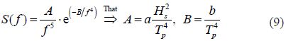
The above scenario is repeated just by using ITTC spectrum. For the spectrum, a general form is assumed as below:
This results in calibration of constants a and b for the spectrum as reported in Table 6 for the case of direction sensitive calibration and one model for each station and /or direction.
| Model | Extreme event direction | a | b | R2 | A/m2 | /Hz | |
| St and ard ITTC model | West-Northwest | 0.31 | 1.25 | 0.11 | 0.83 | 0.003 | 0 |
| West | 0.31 | 1.25 | 0.09 | 0.82 | 0.002 | 0 | |
| South-Southwest | 0.31 | 1.25 | 0.10 | 0.90 | 0.002 | 0 | |
| Southeast | 0.31 | 1.25 | 0.10 | 0.85 | 0.003 | 0 | |
| Calibrated ITTC model | West-Northwest | 0.33 | 1.22 | 0.02 | 0.95 | 0.001 | 0 |
| West | 0.34 | 1.26 | 0.02 | 0.94 | 0.001 | 0 | |
| South-Southwest | 0.28 | 1.20 | 0.03 | 0.93 | 0.001 | 0 | |
| Southeast | 0.29 | 1.22 | 0.04 | 0.90 | 0.001 | 0 |
In this case, the calibration procedure has been also successful when considering NErrordecline of more than 80% at West-Northwest event direction as well as R2 increase of up to 10% again West-Northwest event direction. Besides, the calibration procedure plays a beneficial role at all other stations even with such a small change in constant coefficients.
For the fully calibrated ITTC model the results are presented in Table 7 together with its ancestor st and ard ITTC model performance in the case of treating all data irrespective of their directions.
| Model | a | b | N Error | R2 | ΔA/m2 | Δfp/Hz |
| St and ard ITTC model | 0.31 | 1.25 | 0.10 | 0.86 | 0.002 | 0 |
| Fully calibrated ITTC model | 0.30 | 1.22 | 0.04 | 0.90 | 0.001 | 0 |
Fig. 11 shows the great change in ITTC performance as developed from a st and ard version to a calibrated version. It is also evident that the conformity has been weakened in the case of direction insensitive version when compared with its direction sensitive version for the sake of simplicity.

|
| Fig. 11 Comparison of an observed spectrum with different versions of ITTC model for a typical West-Northwest wave of Hs=1.30 m and Tp=5.27 s |
The calibrated ITTC model is introduced as the most successful c and idate for the region under this study. The three field spectra with different sea states and direction are presented in Fig. 12. Considering statistical measures of calibrated ITTC and fully calibrated ITTC, it could be shown that the fully calibrated version performs better in the West direction as it is also obvious from reviewing such figures. It performs good enough to encourage one using the same formulation for all directions.

|
| Fig. 12 Comparison of an observed spectrum with different versions of ITTC model |
To provide a wider scope on achievements, this section aims at reviewing results from another angle. In other words, the maximum value of spectral value had not been directly taken into account when performing calibration. In Figs. 13 and 14, such peak values(Smax)are extracted for st and ard, direction sensitive and direction insensitive calibrated version of both JONSWAP and ITTC.

|
| Fig. 13 Predicting peak value(Smax)of wave spectrum; st and ard, calibrated and fully calibrated JONSWAP spectral model |

|
| Fig. 14 Predicting peak value of wave spectrum; st and ard, calibrated and fully calibrated ITTC spectral model |
It is evident that all versions of ITTC model predict peak values with less variance. Besides, fully calibrated versions of both JONSWAP and ITTC improve the situation on prediction of peak values even in comparison with their calibrated version. Although, this is not the case when looking at their performance based on NError and R2, but they clearly fall behind their calibrated versions. Besides, they interestingly have exactly a similar performance in predicting peak values.
5 ConclusionsIn this study spectra at four distinct stations at the Strait of Hormuz was observed and studied with respect to performance of st and ard well-known spectra to model the region. Results showed that the st and ard ITTC model is more appropriate at the regions when compared with PM and JONSWAP models. This is in contrast to what is now implemented by designers. Therefore, ITTC spectrum should be used in order to have a more precise model of the region.
The calibrated procedure with respect to four recognized directions in which each was related to one station at the region using GRG algorithm resulted in greater conformity between calibrated ITTC and measurements. However, one consisted of having four models for four stations which is a little bit unpractical. Therefore, a second try in calibration was conducted for all recorded data irrespective of stations and /or directions to introduce the fully calibrated version of ITTC. This new version covered the whole area under study irrespective of direction. It also introduced as the best practical spectrum, although it is weaker in terms of statistical performance when compare with that of first calibration outputs.
In this paper, peak frequency treated as a direct input of ITTC is based on observed data. This is a great subject for future research. It could be used to provide an equation for a parameter with respect to other quantities while a relation between significant wave height and peak period presented in this research, which is evidently different from those of other seas.
| Abadie J (1978). The GRG method for nonlinear programming. In: HJ Greenberg (ed.) Design and Implementation of Optimization Software. Sijthoff and Noordhoff, Alphen aan den Rijn, Netherlands, 335-363. |
| Akers B, Nicholls DP (2012). Spectral stability of deep two-dimensional gravity water waves: repeated eigenvalues. Journal of Applied Mathematics, 72(2), 689-711. DOI: 10.1137/110832446 |
| Akers B, Nicholls DP (2014). The spectrum of finite depth water waves. European Journal of Mechanics, 46, 181-189. DOI:10.1016/j.euromechflu.2014.03.010 |
| Akhmediev N, Soto-Crespo JM, Devine N, Hoffmann NP (2015). Rogue wave spectra of the Sasa-Satsuma equation. Nonlinear Phenomena, 294, 37-42. DOI: 10.1016/j.physd.2014.11.006 |
| Belibassakis KA, Athanassoulis GA, Gerostathis TP (2014). Directional wave spectrum transformation in the presence of strong depth and current inhomogeneities by means of coupled-mode model. Ocean Engineering, 87, 84-96. DOI: 10.1016/j.oceaneng.2014.05.007 |
| Casas Prat M (2009). Overview of ocean wave statistics. Bachelor's thesis, University of Catalunia, Barcelon, 3-12. |
| Chakrabarti SK (2005). Handbook of offshore engineering. 1st ed., Elsevier, Amsterdam, 275-293. |
| Eldeberky Y (2011). Modeling spectra of breaking waves propagating over a beach. Ain Shams Engineering Journal, 2(2), 71-77. DOI: 10.1016/j.asej.2011.07.002 |
| Hasselmann K, Barnett TP, Bouws E, Carlson H, Cartwright DE, Enke K, Ewing JA, Gienapp H, Hasselmann DE, Kruseman P, Meerburg A, Müller P, Olbers DJ, Richter K, Sell W, Walden H (1973). Measurements of wind-wave growth and swell decay during the Joint North Sea Wave Project (JONSWAP). Deutschen Hydrographic Institute, Hamburg, Technical Report No 551.466.31. |
| ITTC (2002). The specialist committee on waves. 23rd International Towing Tank Conference, Venice, Italy, 544-551. |
| Kuik AJ, Van Vledder GP, Holthuijsen LH (1988). A method for the routine analysis of pitch-and-roll buoy wave data. Journal of Physical Oceanography, 18(7), 1020-1034. DOI:10.1175/15200485(1988)018%3C1020:AMFTRA%3E2.0.CO;2 |
| Kumar VS, Kumar KA (2008). Spectral characteristic of high shallow water waves. Ocean Engineering, 35(8-9), 900-911. DOI: 10.1016/j.oceaneng.2008.01.016 |
| Lucas C, Boukhanovsky A, Guedes Soares C (2011). Modeling the climatic variability of directional wave spectra. Ocean Engineering, 38(11-12), 1283-1290. DOI: 10.1016/j.oceaneng.2011.04.003 |
| Manzano-Agugliaro F, Corchete V, Lastra XB (2011). Spectral analysis of tide waves in the Strait of Gibraltar. Scientific Research and Essays, 6(2), 453-462. |
| Mazaheri S, Ghaderi Z (2011). Shallow water wave characteristics in Persian Gulf. Journal of Coastal Research, Special Issue 64(1), 572-575. |
| Ochi MK, Hubble EN (1976). Six-parameter wave spectra. Proceedings of the 15th Coastal Engineering Conference, Honolulu, USA, 301-328. DOI: 10.9753/icce.v15.%25p |
| Parvaresh A, Hassanzadeh S, Bordbar MH (2005). Statistical analysis of wave parameters in the north coast of the Persian Gulf. Annales Geophysicae, 23(6), 2031-2038. DOI: 10.5194/angeo-23-2031-2005 |
| Pierson Jr WJ, Moskowitz L (1964). A proposed spectral form for fully developed wind seas based on the similarity theory. Journal of Geophysical Research, 69(24), 5181-5190. DOI: 10.1029/JZ069i024p05181 |
| Srisuwan C, Work PA (2013). Directional surface wave spectra from acoustic Doppler current profiler data in sheared and stratified flows. Ocean Engineering, 72, 149-159. DOI: 10.1016/j.oceaneng.2013.06.003 |
| Tanaka M, Yokoyama N (2004). Effects of discretization of the spectrum in water-wave turbulence. Fluid Dynamics Research, 34(3), 199-216. DOI: 10.1016/j.fluiddyn.2003.12.001 |
| Tolman HL, Krasnopolsky VM, Chalikov DV (2005). Neural network approximations for nonlinear interactions in wind wave spectra: direct mapping for wind seas in deep water. Ocean Modelling, 8(3), 253-278. DOI: 10.1016/j.ocemod.2003.12.008 |
| Violante-Carvalho N, Parente CE, Robinson IS, Nunes LMP (2002). On the growth of wind-generated waves in a swell-dominated region in the South Atlantic. Journal of Offshore Mechanics and Arctic Engineering, 124(1), 14-21. DOI: 10.1115/1.1423636 |
| Wang YG (2014). Calculating crest statistics of shallow water nonlinear waves based on standard spectra and measured data at the Poseidon platform. Ocean Engineering, 87, 16-24. DOI: 10.1016/j.oceaneng.2014.05.012 |
| Wen F (2011). Study of fully developed wind wave spectrum by application of quantum statistics. Physica A: Statistical Mechanics and its Applications, 390(21), 3855-3869. DOI: 10.1016/j.physa.2011.05.030 |
| Yilman N (2007). Spectral characteristics of wind waves in the eastern Black Sea. PhD thesis, Middle East Technical University, Ankara, Turkey, 47-51. |
| Young IR (1998). Observations of the spectra of hurricane generated waves. Ocean Engineering, 25(4), 261-276. DOI: 10.1016/S0029-8018(97)00011-5 |
| Zahibo N, Didenkulova I, Kurkin A, Pelinovsky E (2008). Steepness and spectrum of nonlinear deformed shallow water wave. Ocean Engineering, 35(1), 47-52. DOI: 10.1016/j.oceaneng.2007.07.001 |