1 Introduction

When a structure in contact with fluid vibrates, there is an interaction between the fluid and the structure. It is called fluid-structure interaction. Different methods should be applied to models with different levels of interaction. The structure in contact with low density fluid is a weak coupled problem, while the structure in contact with high density fluid, such as water, is a strong coupled problem. To solve the strong coupled system, a coupled method should be applied. The fluid-structure interaction level of a plate can be decided by the empirical formulation(Atalla and Bernhard, 1994).

When a structure in contact with fluid vibrates in low frequencies, the fluid is considered as irrotational ideal fluid under small linear load. If the fluid is compressible, then the governing equation of sound pressure or velocity potential is Helmholtz differential equation. In low frequency, the effect of fluid on structure is considered as an added mass effect(Wang et al., 2014). FEM/FEM and FEM/BEM are common methods for solving the vibration characteristics of fluid-structure systems.

Usually, when the structure is closed and the fluid domain is unbounded, FEM/Direct-BEM is an appropriate method(Everstine and Henderson, 1990; Everstine, 1991; Yao et al., 2004). It is easy to use the calculated added mass matrix by Direct-BEM to build system equation, but it can only solve closed structure and the interior or exterior problem needs to be solved separately. Another difficulty in Direct-BEM is the singular integral. When the structure is open and the fluid domain is unbounded, FEM/Indirect-BEM is a widely used method(Coyette and Fyfe, 1989; Jeans and Mathews, 1990; Vlahopoulos et al., 1999; Wei et al., 2011; Liu et al., 2014). There are two advantages to calculate the added mass matrix by Indirect-BEM. The first is that it can solve the interior and exterior problem simultaneously. The second is that the obtained matrix is symmetric so that the fluid equation and the structure equation can be coupled better. However, it costs more time to build the system matrix. And it is difficult to deal with the hypersingular integral in Indirect-BEM. FEM/FEM is usually applied to analyze the vibration characteristics of structure in bounded fluid(Gladwell, 1966; Petyt et al., 1976; Volcy et al., 1979; Lu and Clough, 1982; Wang et al., 1988; Everstine, 1997; Tong and Liu, 1997; Zheng et al., 1998; Ahlem, 2004; Thompson, 2005; Yao et al., 2006; Wu and Zhao, 2007; Zhao et al., 2007). The advantage of calculating the added mass matrix by FEM is that the obtained fluid mass and stiffness matrices are symmetric, sparse and real matrices. It is easier to compute the matrices using FEM than Direct-BEM or Indirect-BEM. For large scale exterior problems the FEM/FEM needs lower computational cost. FEM has no singular integral. And the obtained fluid mass and stiffness matrices are irrelevant to the vibrating frequency so that they need not to be computed repeatedly. BEM doesn’t have these advantages. Experiments are often used to verify the numerical results obtained by FEM/FEM or FEM/BEM(Volcy et al., 1979; Chen et al., 1999; Chen et al., 2003; Liu et al., 2014).

This paper presents a numerical method for calculating the added mass of structure that is in bounded fluid in low frequency. After adding the added mass matrix to the structure mass matrix, a fluid-structure interaction mass matrix is obtained. Combining the matrix with structure stiffness matrix, the generalized characteristic equation of the system is attained. The vibration characteristics of the system are calculated by solving the equation. In this paper, a FORTRAN code is programmed that computes the vibration characteristics of structure in the bounded fluid domain. The cantilever plate example demonstrates that fluid changes the structure’s dynamic characteristics. A verification experiment based on a loaded ship model is performed and the results show good correlation with the numerical solutions. The derivation of numerical method for the fluid-structure has a good reference value to the research of fluid-structure dynamics and acoustic radiation.

2 Basic theories 2.1 Derivation of Helmholtz integral equation in fluid domain

As shown in Fig. 1, V is the bounded fluid domain and $\Omega$ is its boundary. When the structure in contact with the fluid vibrates, the vibration has an effect on fluid, which produces a radiation sound pressure filed in the fluid domain. The sound pressure in the fluid domain also has an effect on the structure in return. For the irrotational, compressible fluid, under the small linear load, the pressure p in the fluid domain satisfies Helmholtz differential equation:

where $k=\omega /c$ is the wave number, Ω the angular frequency and c the sound velocity in fluid.

For Eq.(1), the weighted integral form in the fluid domain is:

where w is the weighted function.

Using integration by parts, Eq.(2)becomes:

where $\int\limits_{V}{\nabla w\nabla p\text{d}V}=\int\limits_{V}{\left(\frac{\partial w}{\partial x}\frac{\partial p}{\partial x}+\frac{\partial w}{\partial y}\frac{\partial p}{\partial y}+\frac{\partial w}{\partial z}\frac{\partial p}{\partial z} \right)}\text{d}V$.

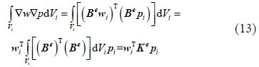
According to the Gaussian divergence theorem, the first term of Eq.(3)becomes:

where ${{\rho }_{0}}$ is the fluid density, v is the particle velocity vector and n the unit normal of the fluid boundary.

Substituting Eq.(4)into Eq.(3), Eq.(5)is obtained as follows:

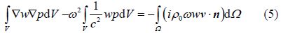
Eq.(5)is the Helmholtz integral equation over the fluid domain and boundary. It’s the theoretical basis to solve Helmholtz differential equation.

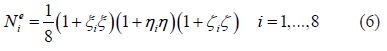
2.2 Solving Helmholtz integral equation of the fluid domain by FEM

This paper uses 8-nodes isoparametric hexahedral element to discretize the bounded fluid domain, as shown in Fig. 2. The shape function of 8-nodes isoparametric hexahedral element is:

The corresponding coordinate is shown in Fig. 2.

The discrete form of Eq.(5)is

where n_f is the number of fluid elements, and n the number of fluid boundary elements.

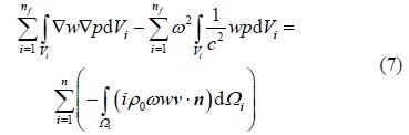
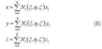
For 8-nodes isoparametric hexahedral element, coordinates transformation using the same shape function can satisfy the compatibility dem and :

The weighted function at any point in an element can be interpolated by the shape function:

The sound pressure at any point in an element can be interpolated by the shape function:

For Eq.(7), the first term on the left is $\sum\limits_{i=1}^{{{n}_{f}}}{\int\limits_{{{V}_{i}}}{\nabla w\nabla p\text{d}{{V}_{i}}}}$, according to Eq.(9) and Eq.(10):

where

${{B}^{e}}=\left[ \begin{matrix} \frac{\partial {{N}_{1}}}{\partial x} & \frac{\partial {{N}_{2}}}{\partial x} & \frac{\partial {{N}_{3}}}{\partial x} & \frac{\partial {{N}_{4}}}{\partial x} & \frac{\partial {{N}_{5}}}{\partial x} & \frac{\partial {{N}_{6}}}{\partial x} & \frac{\partial {{N}_{7}}}{\partial x} & \frac{\partial {{N}_{8}}}{\partial x} \\ \frac{\partial {{N}_{1}}}{\partial y} & \frac{\partial {{N}_{2}}}{\partial y} & \frac{\partial {{N}_{3}}}{\partial y} & \frac{\partial {{N}_{4}}}{\partial y} & \frac{\partial {{N}_{5}}}{\partial y} & \frac{\partial {{N}_{6}}}{\partial y} & \frac{\partial {{N}_{7}}}{\partial y} & \frac{\partial {{N}_{8}}}{\partial y} \\ \frac{\partial {{N}_{1}}}{\partial z} & \frac{\partial {{N}_{2}}}{\partial z} & \frac{\partial {{N}_{3}}}{\partial z} & \frac{\partial {{N}_{4}}}{\partial z} & \frac{\partial {{N}_{5}}}{\partial z} & \frac{\partial {{N}_{6}}}{\partial z} & \frac{\partial {{N}_{7}}}{\partial z} & \frac{\partial {{N}_{8}}}{\partial z} \\ \end{matrix} \right]$

Substituting Eq.(11) and Eq.(12)into $\sum\limits_{i=1}^{{{n}_{f}}}{\int\limits_{{{V}_{i}}}{\nabla w\nabla p\text{d}{{V}_{i}}}}$:

where K^e is a matrix of 8×8:

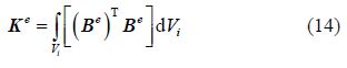
Transforming Eq.(14)to the integral form under the local coordinate system:

where |J| is the Jacobi determinant with the following form:

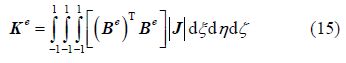
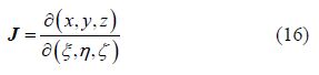
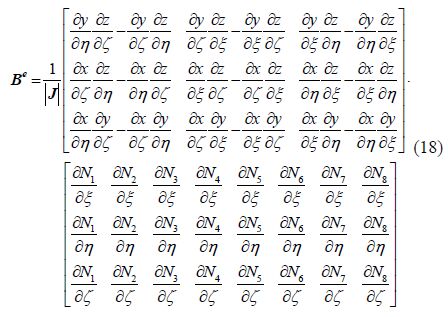
Considering the form of B^e, it needs to be transformed from global coordinate system to local coordinate system before integration:

For Eq.(7), the second term on the left is $-\sum\limits_{i=1}^{{{n}_{f}}}{{{\omega }^{2}}\int\limits_{{{V}_{i}}}{\frac{1}{{{c}^{2}}}wp\text{d}{{V}_{i}}}}$, substituting Eq.(9) and Eq.(10)to Eq.(19):

where N is the shape function vector and M^e is a matrix of 8x8:

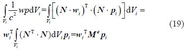
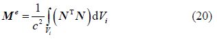
The integral form of Eq.(20)in local coordinate system is:

2.3 Solving the fluid-structure vibration characteristics problem by combining structure FEM and fluid FEM

The right-h and side of Eq.(7)is $\sum\limits_{i=1}^{n}{\left(-\int\limits_{{{\Omega }_{i}}}{\left(i{{\rho }_{0}}\omega wv\cdot n \right)\text{d}{{\Omega }_{i}}} \right)}$. The integral boundary Ωcan be divided into velocity boundary Ω_v, acoustic impedance boundary Ω_z and pressure boundary Ω_p, as shown in Fig. 3.

Considering the derivation in Section 2.2, the governing equation of the acoustic field in FEM form is:

where K_a is the stiffness matrix of the whole fluid, M_a is the mass matrix of the whole fluid, F_a is the effect of the boundary conditions of acoustic field, including the velocity boundary Ω_v, the acoustic impedance boundary Ω_z and the pressure boundary Ω_p.

For the fluid-structure vibration characteristics problems, the normal velocity of structure is equal to fluid velocity in the coupled interface between fluid and structure. It is shown in Fig. 4.

Without the damping effect, the structural motion equation in the FEM form is:

where K_sis the stiffness matrix of the whole structure, M_s the mass matrix of the whole structure, u the displacement vector of the structure and F_s the load vector on the structure.

The sound pressure p, which is perpendicular to the fluid-structure interface, satisfies the following:

where n_se is the number of the elements at fluid-structure interface, n^e is the normal vector of the element, N^s is the shape function of the structure element, N^a is the shape function of the fluid element, Ω_se is the fluid-structure interface.

Considering the fluid-structure interaction, sound pressure acting on the structure can be seen as added normal loads. Combining Eq.(23) and Eq.(24), the structural motion equation considering fluid-structure interaction is:

where K_c is the fluid-structure coupling stiffness matrix:

On the fluid-structure interface, the velocity of structure can be seen as the boundary conditions of sound field. Using Eq.(22), the sound field equation considering fluid-structure interaction is

where M_c is the fluid-structure coupling mass matrix:

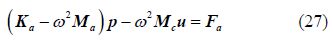
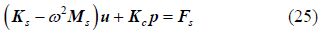
Combining Eq.(25) and Eq.(27), the fluid-structure interaction motion equations based on FEM theory is:

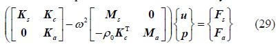
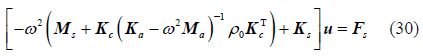
If fluid-structure interaction boundary is the only boundary(${{\mathbf{F}}_{a}}=0$), then p can be deleted in Eq.(29):

The corresponding equation of generalized eigenvalue problem is:

where ${{M}_{add}}={{\rho }_{0}}{{K}_{c}}{{\left( {{K}_{a}}-{{\omega }^{2}}{{M}_{a}} \right)}^{-1}}K_{c}^{T}$ is the structural added mass matrix, M_add is a real symmetric b and matrix.

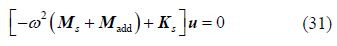
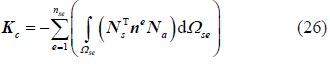
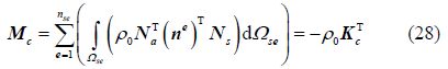
The fluid-structure coupling matrix K_c is related to the element normal vector n^e. If there is only one fluid domain, as shown in Fig. 5(a), the normal vector n^e of boundary element can either point into the fluid or point away from the fluid, and all the elements should be consistent. From the form of M_add, it can be found that it includes K_c and $K_{c}^{\text{T}}$. Therefore, for a multi-fluid domain problem, as shown in Fig. 5(b), the element normal vectors n^eof each fluid domain(V₁, V₂, V₃ or V₄)should be consistent.

A FORTRAN program is developed to calculate the vibration characteristics of structure under fluid load and air load based on the fluid and structure finite element method theory. The program flow chart is shown in Fig. 6. Flow diagram in the dotted box is used for calculating air loaded ship model.

3 Numerical examples

For elastic cantilever plate submerged in bounded fluid domain, boundaries of the fluid domain are shown in Fig. 7. The length of the plate a is 0.50 m, width b is 0.30 m and thickness t is 0.004 m. The Poisson ratio of the material is 0.3, the Young's modulus is  N/m² and the plate’s density is 7 800 kg/m³.

Assuming that the fluid is compressible, the fluid density is 1 000 kg/m³, and the sound velocity is 1 500 m/s. The upper surface of the fluid domain is free surface, so it has the boundary condition p=0. The other five surfaces of the fluid domain are rigid surfaces, so they have the boundary condition v=0. The vibration characteristics of cantilever plate submerged at three different depths shown in Fig. 8 are calculated. The calculated fundamental frequencies of the cantilever plates are shown in Table 1.

It can be seen that the results shown in Table 1 and Fig. 9 are consistent with the results in Volcy et al.(1979) and Wang et al.(1988).

4 Experimental researches

To verify the derived numerical method and the validity of the FORTRAN program in this paper, modal identification experiments were conducted for a full free ship model in the water and air under different loads.

4.1 Introduction to the experimental model and instrument

The ship model’s length, width, moulded depth and steel plate thickness are 1.50, 0.30, 0.15 and 0.005 m. Fig. 10 shows the experiment that was done in the Ship Structure Vibration Laboratory and towing basin in Dalian University of Technology. The laboratory instruments included a DH5922 dynamic signal analysis instrument, ICP acceleration sensors, and so on.

4.2 Numerical analysis of the experiment model

In this paper, using the dynamic analysis FORTRAN program for fluid-structure interaction problems, free modes of the loaded ship model are calculated. The Poisson ratio of the material is 0.3, the Young modulus 2.1x10¹¹ N/m², and the density 7 800 kg/m³. The loaded water on the ship model is regarded as compressible fluid. Its density is 1 000 kg/m³ and the sound velocity is 1 500 m/s. The calculated frequency for the added mass matrix is 100 Hz. The meshes of the ship model and fluid are shown in Fig. 11. The boundary condition of the free surface of the fluid is set as p=0, and the boundary condition of rigid towing basin side walls and bottom is set as v=0.

4.3 The experiment model measurement

The schematic diagram of the modal identification experiment is shown in Fig. 12. The excitation on the ship model is a pulse type. The arrangement of the eleven acceleration sensors is shown in Fig. 13. Through the modal identification experiment, the ship model’s bending modes, including modal shapes and natural frequencies, can be measured.

4.4 Comparison of results

Numerical results of the ship model under seven load conditions are compared in the experiment. Fig. 14 compares the experimental and numerical modal shapes of the full free ship model. The first two order natural bending modal shapes under different loads in the air and in the fluid are presented, where the cloud maps on the left are the numerical modal shapes and the fitted curves on the right are the corresponding experimental modal shapes.

The first two order natural frequencies of loaded ship model’s bending modes in the air are shown in Table 2 and Fig. 15. The natural frequencies in water are shown in Table 3 and Fig. 16.

From Table 2, Table 3 and Fig. 14, it can be seen that the numerical results of the vibration modes of the ship model, are well consistent with the modal identification experiment results using the method derived in this paper. The results verify the method and the program. Comparing the load conditions 2 and 3 in the air and in the water, or comparing the load conditions 4, 5, 6 and 7, it can be determined that the locations of the loads have an effect on the structure vibration characteristics when the load quantity is constant. Comparing the load condition 2 and 4 or comparing the load condition 3 and 5 in the air and in the water, it can also be seen that the change of the load quantity has little effect on natural frequencies of the structure.

5 Conclusions

Based on the Helmholtz differential equation, the added mass matrix of the structure in bounded fluid domain is derived in low frequency. Considering the fluid compressibility, the vibration characteristics of the cantilever plate submerged at different depth are calculated. The different loaded ship models’ vibration characteristics in the air and in the fluid are also calculated. Finally, a modal identification experiment of a ship model is performed. Several conclusions are drawn below.

The method of deriving the structure adding mass matrix is simple and highly accurate. It has some benefits for calculating the fluid-structure interaction vibration characteristics and acoustic radiation characteristics.

Regarding the modal identification experiment of the structure in bounded fluid domain, the identified result can be influenced by a lot of factors, such as the position and the magnitude of the excitation, load condition and the outside interference signal.

From the modal identification experiment of the ship model under different load conditions, it can be seen that different locations of loads can influence the vibration characteristics of the structure in contact with fluid and the growth of load quantity probably has not a significant influence on the vibration characteristics of the structure.