


 ,
,
2. Defence Science and Technology Organization, Edinburgh, SA, 5111, Australia
1 Introduction
A method for solving the flow field around a fully-submerged object moving near the free surface was put forward by Havelock(1932). The method uses modified sources distributed over the surface of the body. As the method was formulated before the development of computers, no numerical results were calculated for general hull shapes using the method. However, equations were provided for the source potential which automatically satisfies the linearized free-surface boundary condition. These sources will be referred to as “Havelock sources”, following Tuck et al.(2002).
With the advent of computers, Hess and Smith(1964) developed a panel method for a non-lifting body in an unbounded fluid using omnidirectional (Rankine) sources. The body is discretised into panels, each of which has uniform source density. The benefits of this method are that analytical expressions exist for the velocity field produced by each panel, and the resulting velocity field is non-singular, when using distributed sources rather than point sources.
At the time of publication of Hess and Smith’s panel method, naval architects were searching for a new method of ship wave resistance prediction as an improvement over the thin-ship theory of Michell(1898). Bhattacharyya(1965) combined the Hess and Smith(1964) panel method with the potential formulation for Havelock sources as a means of calculating ship wave resistance. Such an approach was subsequently followed by many authors, as reviewed in Noblesse et al.(2013). This problem is called the Neumann- Kelvin problem, as it uses an exact (Neumann) hull boundary condition with a linearized (Kelvin) free surface boundary condition.
For surface ships, except perhaps SWATH ships, the Neumann-Kelvin problem is inconsistent, as linearization of the free surface boundary condition implies a ship with small beam-length ratio, for which the hull boundary condition may also be justifiably linearized. When integrating Havelock sources up to the free surface, care must be taken with the singularity that occurs at the still water level.
For submarines the difficulties described above are essentially removed. Contemporary naval submarines have a non-negligible diameter-to-length ratio in the order of 1:7 to 1:12 and a large stagnation area at the bow. As a result, a nonlinear hull boundary condition is desirable. However, when fully submerged, submarines produce only a small disturbance on the free surface and the free surface boundary condition can be justifiably linearized. Also, since every part of the hull lies beneath the free surface, the Havelock source potential is finite everywhere except at the source.
The Havelock source panel method has been applied to submerged spheroids by Farell(1973), Guével et al.(1977), Hong(1983) and Doctors and Beck(1987b), and we shall make comparisons with the latter predictions in this article.
Other methods in use for modelling flow around near- surface submarine hulls include nonlinear Rankine-source panel codes (Flowtech International AB, 2012) and RANS-CFD codes, each of which are used to a limited extent in Dawson(2014).
2 Single Havelock sourceWe use a body-fixed coordinate system in which x is positive forward, y is positive to port and z is positive upwards, as shown in Fig. 1.

|
| Fig. 1 Body-fixed coordinate system for a Havelock point source |
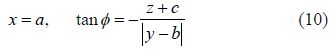
Accurate calculation of the velocity potential due to a single Havelock source is not a trivial task. It is likely that this is the reason for the large scatter in predictions presented by different authors, as discussed for surface ships in Doctors and Beck(1987a) and as discussed for submerged spheroids in Doctors and Beck(1987b). The basic formulation for a Havelock source is given by Havelock(1932) and Wehausen and Laitone(1960) and involves a singular and highly-oscillatory double integral. Here we use the more computationally amenable method developed by Noblesse(1981) and given in Newman(1987). In our coordinate system, the velocity potential Φ due to a single positive source of strength 4π at(a, b, c) moving at speed U is:

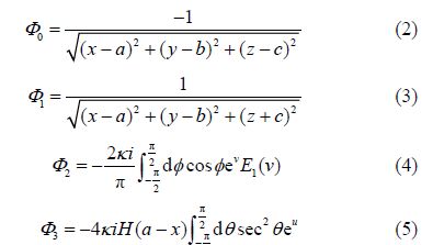
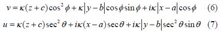
The arguments in (4) and (5) are:
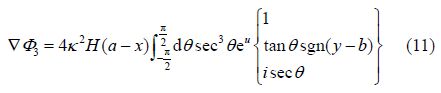
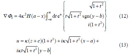
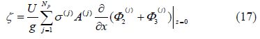
The term Φ0 is the st and ard Rankine source positioned at (a, b, c). The term Φ1 is an equal sink positioned above the free surface at (a, b, −c). The term Φ2 we shall call the “near-field” term as it is only important close to the source. The last term Φ3 we shall call the “far-field” term as it is important everywhere downstream of the source and is responsible for the wave-like free surface.
The dynamic free surface boundary condition may be linearized to give the free surface height ζ due to a single Havelock source as:
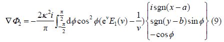
The $(\hat x,\hat y,\hat z)$ velocity components of the near-field term are given by:
The $(\hat x,\hat y,\hat z)$ velocity components of the far-field term are given by:
Consider a single Havelock source with strength 4π m3/s, as given by (1), lying 10 m beneath the free surface and moving at 5 m/s. The longitudinal velocity produced at (x, y, z) = (x, 0, 0) for this Havelock source is shown in Fig. 2.

|
| Fig. 2 Longitudinal flow velocity (m/s) produced by a single Havelock source |
On the free surface, the longitudinal velocity components due to Φ0 and Φ1 cancel one another. The total velocity field is continuous across x=0, despite the fact that the near-field component Φ2 and far-field component Φ3 are each discontinuous across x=0. This serves as a useful check on the accuracy of the independently calculated Φ2 and Φ3.
3 The Havelock source panel methodThe coordinate system and principal submarine dimensions used for the Havelock source panel method are shown in Fig. 3.

|
| Fig. 3 Coordinate system and submarine dimensions for the Havelocksource panel method |
The panel method approach described here for a near-surface body follows closely that of Hess and Smith(1964) for a body in an unbounded fluid. In that method, the sources used are Rankine sources, that is, the component Φ0 in Eq.(1). Here we follow the method of Hess and Smith but include the additional terms Φ1, Φ2, Φ3.
The body is first discretised into Np triangular and /or quadrilateral panels of area A(j) and unknown source density σ(j), such that:
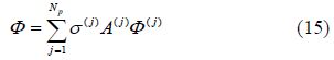
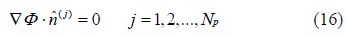
When calculating the velocity potential due to each panel Φ(j), the inclusion of the image source term Φ1 is straightforward, as each panel vertex can be reflected about the free surface and the analytic expressions for the flow velocity induced by each panel remain unchanged from those given in Hess and Smith(1964).
The expressions for Φ2 and Φ3, like Φ1, depend on the position vector from the image source, as shown in Fig. 4. For fully-submerged hulls, the receiver panel is generally a large distance from the image panel (relative to the panel dimensions), so we may approximate the image panel as a point source of strength (<source density><panel area>). This conclusion was also reached by Doctors and Beck(1987b). Therefore the expressions for Φ2 and Φ3 are evaluated as point sources, which simplifies the analysis.

|
| Fig. 4 Havelock source panel method. Calculation of Φ0is based on vector from hull source panel to receiver panel. Calculation ofΦ1, Φ2, Φ3 is based on vector from image source panel to receiver panel. Example shows DARPA SUBOFF hull with sail near free surface. |
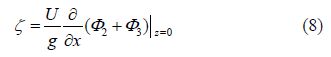
Having solved for the source strengths and flow velocities as described above, further outputs can be computed. Eqs.(8) and (15) may be combined to yield the total wave pattern as:


In practice the pressure drag and wave resistance generally show close agreement; however, the pressure drag given by Eq.(21) is slower to converge and more erratic at low Froude numbers than the far-field wave resistance given by Eq.(22). For this reason we tend to use Eq.(22) to calculate the resistance due to wave making in the near-surface submergence condition.
The Havelock source panel method described here is implemented in a computer code entitled “HullWave” developed at the Centre for Marine Science and Technology, Curtin University. The code is written in MATLAB (The Mathworks, 2014) and runs on a st and ard desktop PC. Run times for the Joubert hull with Np=800 in the near-surface condition (see Section 8) were 15 minutes for each speed on an Intel i7-940 2.93 GHz processor with 12 GB of RAM. Runs may be split across multiple cores to quickly do a range of speeds.
4 Comparison with experiments for a deeply-submerged DARPA SUBOFF submarine hullOffsets for the DARPA SUBOFF st and ard series submarine hull are given in Groves et al.(1989). This is shown in Fig. 5 together with the other st and ard-series hulls analysed in this report, namely the Series 58 models 4165 and 4166 (Gertler, 1950) and DSTO Joubert models with length-to-diameter ratios 7.3, 8.5 and 9.5 (Dawson, 2014).

|
| Fig. 5 Comparative geometries of st and ard-series submarine hulls used for analysis |
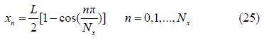
Predictions using the present method for a deeply- submerged DARPA SUBOFF hull will be compared with measured surface pressures from wind tunnel tests described in Huang et al.(1994). For a deeply submerged submarine, the Havelock source panel method described here reverts to the st and ard Hess and Smith(1964) panel method. A comparison of predicted and measured cp values is shown in Fig. 6. The predicted results given here use a grid of 100 panels longitudinally (Nx=100) and 25 panels circumferentially from the bottom to the top (Ng=25), giving a total of 2 500 panels on each side (Np=2 500). Gridlines are clustered longitudinally toward the ends using cosine spacing, that is:

|
| Fig. 6 Pressure coefficient on DARPA SUBOFF bare hull, using HullWave panel method in deep-submergence condition and experimental wind tunnel results from Huang et al.(1994). |
We see that the pressure is quite well predicted over most of the hull. However, near the stern of the submarine (0≤x/L≤0.1) the effects of boundary layer thickening and separation cause a lower pressure in the experiments than is predicted using the present inviscid theory. Further differences, which cannot be explained by the neglect of viscosity, are observed close to the bow.
5 Convergence testing for a near-surface spheroidIn order to check the present method’s convergence with increasing number of panels, a 5:1:1 prolate spheroid is analysed at very shallow submergence H/D=0.8 and the high Froude number FL=0.8. Panels were evenly spaced in the circumferential direction, with cosine spacing in the longitudinal direction as in (25). The ratio between longitudinal and circumferential panels was Nx/Ng=4, as used by Doctors and Beck(1987b, Fig. 3). Panel densities of Np=36, 64, 100, 400, 900, 1 600, 2 500, 3 600 were used.
The same configuration was analysed by Doctors and Beck(1987b, Fig. 3) using Havelock sources with two different techniques: a “Panel” technique in which flow velocities are calculated only at the null points of receiver panels (as done by Hess and Smith(1964)); and a “Galerkin” method in which flow velocities are integrated over the receiver panels. Due to the limited computing power available at the time, results were computed for Np=36, 64, 100 and Richardson’s extrapolation technique was used to estimate the fully-converged solution (shown as “extrap.” on the graphs).
Convergence results from the present method and that of Doctors and Beck(1987b, Fig. 3) are shown in Fig. 7 for the lift coefficient, Fig. 8 for the wave resistance coefficient and Fig. 9 for the pressure drag coefficient. The trim moment presented in Doctors and Beck(1987b, Fig. 3) was taken about a different axis, and so cannot be directly compared with the present results. The present results showed good convergence of the trim moment coefficient.

|
| Fig. 7 Convergence test for lift coefficient of submergedD/L=0.2 spheroid at H/D=0.8, FL=0.8. (DB) Results from Doctors and Beck(1987b, Fig. 3c) |

|
| Fig. 8 Convergence test for wave resistance coefficient of submerged D/L=0.2 spheroid at H/D=0.8, FL=0.8. (DB) Results from Doctors and Beck(1987b, Fig. 3b) |

|
| Fig. 9 Convergence test for pressure drag coefficient of submerged D/L=0.2 spheroid at H/D=0.8, FL=0.8. (DB) Results from Doctors and Beck(1987b, Fig. 3a) |
Convergence testing of the present method at H/D=0.8 and FL=0.3 showed good convergence for vertical force, trim moment and wave resistance, but poor convergence for pressure drag.
Comparison was also made with the results given by Doctors and Beck(1987b, Figs. 4, 5) for a 5:1:1 spheroid at H/D=0.8 and H/D=1.225. The present results confirmed the Doctors and Beck(1987b, Figs. 4a, 5a, 5b) results for wave resistance, including at FL<0.4 where Doctors and Beck(1987b) had noted discrepancies with previous studies. The present results also confirmed the lift coefficient across all Froude numbers as given in Doctors and Beck(1987b, Fig. 4b). The trim moment in Doctors and Beck(1987b, Fig. 4c) was taken about the free surface, so could not be directly compared with the present results.
6 Comparison with experiments for a near- surface Series 58 hullCalculations of wave resistance were completed using the Havelock source panel method for Series 58 models 4165 and 4166 (Gertler, 1950). These are compared with model test residuary resistance (Gertler, 1950) in Fig. 10 and Fig. 11. The geometries of the two hulls are shown in Fig. 5. The mesh for each hull had 20 evenly-spaced panels in the circumferential direction and 80 panels with cosine spacing in the longitudinal direction, that is Np=1 600.

|
| Fig. 10 Predicted wave resistance coefficient, together with residuary resistance coefficient from Gertler(1950) experiments, for a Series 58 model 4165 hull with prismatic coefficient 0.65. |

|
| Fig. 11 Predicted wave resistance coefficient, together with residuary resistance coefficient from Gertler(1950) experiments, for a Series 58 model 4166 hull with prismatic coefficient 0.70. |
Gertler(1950) calculated residuary resistance by subtracting the resistance of the towing strut measured in isolation and the frictional resistance calculated using the Schoenherr friction line from the total measured resistance. Small errors in each of these assumptions cause an offset in the plotted residuary resistance, as evidenced at low Froude numbers. Taking this offset into account, we see that the peaks at FL≈0.5 are well-predicted for both hulls.
The model test data shows very different behaviour of the two hulls in the region of the smaller peak at FL≈0.3. The lower-prismatic hull 4165 has low residuary resistance in this region, whereas the high-prismatic 4166 has a noticeable peak at FL≈0.3. This different behaviour is caused by the marked pressure changes at the forward and aft shoulders of the high-prismatic hull.
7 Comparison with experiments for a near- surface DARPA SUBOFF submarine hullCalculations of wave resistance were completed for the DARPA SUBOFF bare hull. These are compared with model test residuary resistance (Dawson, 2014) in Fig. 12. The mesh had 19 evenly-spaced panels in the circumferential direction and 60 panels with cosine spacing in the longitudinal direction, resulting in Np=1 140.

|
| Fig. 12 Predicted wave resistance coefficient (open markers), compared with model test results of residuary resistance coefficient (filled markers) from Dawson(2014), for DARPA SUBOFF bare hull |
Three peaks are evident in predicted and measured wave resistance curves for the shallowest submergence (H/D=1.1). The peaks occur at FL=0.23, 0.29, 0.51. Calculated centreline wave cuts for these Froude numbers are shown in Fig. 13.

|
| Fig. 13 Calculated centreline wave cuts for the DARPA SUBOFF bare hull atH/D=1.1 |
The speed of linear deep-water waves $c = \sqrt {g\lambda /2\pi } $ corresponds to the speed of the submarine at the transverse wavelength $\lambda /L = 2\pi F_L^2$. As seen in Fig. 13, the wave resistance peaks correspond to speeds at which the natural high and low pressure regions around the hull resonate with transverse wave production. At FL=0.23, there is approximately a half-wavelength between the natural high-pressure region at the bow and low-pressure region at the forward shoulder and approximately two wavelengths from there back to the natural low-pressure region at the aft shoulder. At FL=0.29, there are approximately 1.5 wavelengths between the natural high-pressure region at the bow and low-pressure region at the aft shoulder. At FL=0.51, there is approximately one half-wavelength between the natural high-pressure region at the bow and low-pressure region at the aft shoulder.
It should be borne in mind that, as discussed in Dawson(2014), typical operating Froude numbers in the near-surface submerged condition would be unlikely to exceed 0.3 for naval submarines. Therefore predictions and model test results at higher Froude numbers are of lesser relevance to operations of submarines at the present time. Such Froude numbers may be relevant to other craft, such as torpedoes or remote/autonomous underwater vehicles.
Comparisons of predicted wave resistance and measured residuary resistance for the DARPA SUBOFF hull with sail are shown in Fig. 14. The mesh is shown in Fig. 4 and has Np=1 972.

|
| Fig. 14 Predicted wave resistance coefficient (open markers), compared with model test results of residuary resistance coefficient (filled markers) from Dawson(2014), for DARPA SUBOFF hull with sail |
For the DARPA SUBOFF hull with sail, it is seen that the measured residuary resistance agrees quite closely with the calculated wave resistance at the deeper submergences. At the shallowest submergence, the method over-predicts the residuary resistance at all Froude numbers, but especially in the region of the local peak at FL≈0.3. A photograph of the observed free surface at FL=0.31 is shown in Fig. 15, and the calculated centreline wave cut at this speed is shown in Fig. 16.

|
| Fig. 15 Observed wave pattern for the DARPA SUBOFF hull with sail atH/D=1.1 and FL=0.31 |

|
| Fig. 16 Calculated centreline wave cut for the DARPA SUBOFF hull with sail atH/D=1.1 and FL=0.31 |
We see in Fig. 15 that the sail produces its own Kelvin wave pattern, but no ventilation or wave breaking is observed. As calculated in Fig. 16, the sail is very close to the free surface. We expect that the linear wave assumption may break down locally where the hull pierces or comes very close to the free surface. Also, by comparing the measured residuary resistance for the hull and sail with that of the bare hull, we see that the measured residuary resistance for the hull with sail is surprisingly low at the shallowest submergence. Further theoretical and experimental testing with an appended hull would be desirable to better underst and the physics of wave production when the sail is very close to the free surface.
8 Comparison with experiments for a near-surface Joubert submarine hullThe DSTO “Joubert” st and ard-series submarine hulls were extensively tested in the near-surface condition in the work of Dawson(2014). Measurements include vertical lift force, trim moment, resistance and wave elevations. Three length-to-diameter ratio configurations all with a common maximum diameter were tested, as shown in Fig. 5. The model test results for lift coefficient, trim moment coefficient and residuary resistance are compared with predictions from the present theory in Figs. 17-25.

|
| Fig. 17 Predicted lift coefficient (open markers), together with model test results (filled markers) from Dawson(2014), for Joubert hull with L/D=7.3 |

|
| Fig. 18 Predicted trim moment coefficient (open markers), together with model test results (filled markers) from Dawson(2014), for Joubert hull with L/D=7.3 |

|
| Fig. 19 Predicted wave resistance coefficient (open markers), together with residuary resistance coefficient model test results (filled markers) from Dawson(2014), for Joubert hull with L/D=7.3 |

|
| Fig. 20 Predicted lift coefficient (open markers), together with model test results (filled markers) from Dawson(2014), for Joubert hull with L/D=8.5 |

|
| Fig. 21 Predicted trim moment coefficient (open markers), together with model test results (filled markers) from Dawson(2014), for Joubert hull with L/D=8.5 |

|
| Fig. 22 Predicted wave resistance coefficient (open markers), together with residuary resistance coefficient model test results (filled markers) from Dawson(2014), for Joubert hull with L/D=8.5 |

|
| Fig. 23 Predicted lift coefficient (open markers), together with model test results (filled markers) from Dawson(2014), for Joubert hull with L/D=9.5 |

|
| Fig. 24 Predicted trim moment coefficient (open markers), together with model test results (filled markers) from Dawson(2014), for Joubert hull with L/D=9.5 |

|
| Fig. 25 Predicted wave resistance coefficient (open markers), together with residuary resistance coefficient model test results (filled markers) from Dawson(2014), for Joubert hull with L/D=9.5 |
We see that the comparison between predictions and model tests is fairly consistent across all three hulls. Lift force, trim moment and wave resistance are quite closely predicted at typical operating Froude numbers up to 0.3, at all submergences. In the region of the lift force peaks at FL≈0.4 and trim moment and wave resistance peaks at FL≈0.5, the predictions have the correct form but under predict the magnitude.
Predicted near-field wave elevation is shown in Fig. 26, together with model test results from Dawson(2014). In these model tests, the model was held in place by a surface-piercing strut, which affected the wave elevation downstream of the submarine’s stern. Therefore comparisons are only given upstream of the submarine’s stern. We see fairly good agreement between the predicted and measured results, with a slight phase shift in the FL=0.3 case, and a slight over-prediction of the wave elevations in general.

|
| Fig. 26 Wave elevation at y/D=1.26for Joubert hull with L/D=7.3. Experimental results from Dawson(2014) |
A Havelock source panel method for near-surface submerged submarines has been developed by combining the source potential of Havelock(1932) with the panel method of Hess and Smith(1964). The method predicts lift force, trim moment, wave resistance and wave patterns of near-surface submarines, with or without appendages.
The method has been compared with model test data for residuary resistance of two Series 58 hulls, the DARPA SUBOFF hull with and without its sail appendage, and three DSTO Joubert hulls of differing length-to-diameter ratio. The method has also been compared with measured lift force and trim moment of the three Joubert hulls. The simulation results for the SUBOFF and Joubert bare hulls showed close agreement with all measured quantities through the range of typical submarine operating speeds up to FL=0.3. Residuary resistance for the SUBOFF hull with sail agreed well with the simulation predictions except in the extreme near-surface condition. In this instance, additional model testing and theoretical work are desirable to better underst and the differences observed.
In the near field, the method was found to slightly over-predict wave elevations for the Joubert hull, with otherwise good agreement. In the absence of model test data for far-field submarine wave patterns, this aspect of the code has not yet been validated. The computational method as described offers an alternative to RANS-CFD codes, being fast, robust and simple to run.
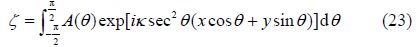
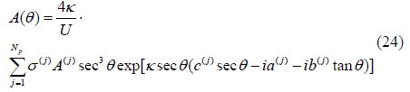
Nomenclature (a(j), b(j), c(j)) (x, y, z)position of null point of jth panelA(θ) Far-field wave amplitude function
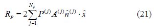
A(j) Area of jth panel
c Wave phase velocity
cD $\frac{{{R_P}}}{{\frac{1}{2}\rho {U^2}S}}$ Pressure drag coefficient
cM $\frac{M}{{\frac{1}{2}\rho {U^2}SL}}$ Trim moment coefficient
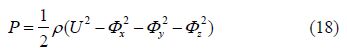
cP $\frac{{P - {P_\infty }}}{{\frac{1}{2}\rho {U^2}}}$ Pressure coefficient
cW $\frac{{{R_W}}}{{\frac{1}{2}\rho {U^2}S}}$ Wave resistance coefficient
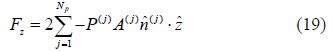
cL $\frac{{{F_Z}}}{{\frac{1}{2}\rho {U^2}S}}$ Lift coefficient
D Maximum hull diameter
E1(v) Exponential integral function, see Abramowitz and Stegun(1965)
FL $\frac{U}{{\sqrt {gL} }}$ Froude number
FZ Hydrodynamic vertical force on submarine, positive upward
g Acceleration due to gravity
H Hull centreline submergence beneath undisturbed free surface
L Submarine hull length
M Hydrodynamic trim moment about midships, positive bow-up
${\hat n^{(j)}}$ Unit outward normal from jth panel
Ng Number of panels circumferentially, from bottom to top on one side
Np Number of panels on one side of hull(2Np panels on entire hull)
Nx Number of panels longitudinally
P Hydrodynamic pressure(pressure above hydrostatic)
P(j) Pressure at null point of jth panel
r Local submarine hull radius
P∞ Hydrodynamic pressure in undisturbed fluid
RP Pressure resistance
RW Wave resistance
S Hull wetted surface area
U Free stream or ship speed
x Body-fixed streamwise coordinate, origin at stern, positive forward
$\hat x$ Unit vector in x direction
y Transverse coordinate, origin at hull centreline, positive to port
ŷ Unit vector in y direction
z Vertical coordinate, origin at still water level, positive upwards
$\hat z$ Unit vector in z direction
κ g/U2
λ Transverse wavelength
ρ Fluid density
ζ Free surface elevation above undisturbed level
σ(j) Source density of jth panel
Φ Velocity potential
Φ(j) Velocity potential due to a single Havelock source at null point of jth panel Acknowledgements
The authors thank the following undergraduate students for their participation in the experimental component of this research: Sam Wilson-Haffenden, Sean Van Steel, Damien Neulist and Nick Johnson.
| Abramowitz M, Stegun IA (1965). Handbook of mathematical functions. Dover Publications, New York. |
| Bhattacharyya R (1965). Uber die berechnung des wellenwiderstandes nach verschiedenen verfahren und vergleich mit einigen experimentellen ergebrissen. Inst. für Schiffbau der Universität Hamburg, Hamburg, Report No. 149. DOI: 10.15480/882.730 |
| Dawson E (2014). An investigation into the effects of submergence depth, speed and hull length-to-diameter ratio on the near-surface operation of conventional submarines. PhD thesis, University of Tasmania, Hobart, Australia. |
| Doctors LJ, Beck RF (1987a). Numerical aspects of the Neumann-Kelvin problem. Journal of Ship Research, 31(1), 1-13. |
| Doctors LJ, Beck RF (1987b). Convergence properties of the Neumann-Kelvin problem for a submerged body. Journal of Ship Research, 31(4), 227-234. |
| Farell C (1973). On the wave resistance of a submerged spheroid. Journal of Ship Research, 17(1), 1-11. |
| Flowtech International AB (2012). SHIPFLOW® 4.7 users manual. Flowtech International, Gothenburg, Sweden. |
| Gertler M (1950). Resistance experiments on a systematic series of streamlined bodies of revolution -for application to the design of high-speed submarines. David Taylor Model Basin, Washington, DC, Report C-297. |
| Gourlay TP (2014). ShallowFlow: a program to model ship hydrodynamics in shallow water. 33rd International Conference on Ocean, Offshore and Arctic Engineering, OMAE 2014, San Francisco, USA, Paper No. OMAE2014-23291. DOI: 10.1115/OMAE2014-23291 |
| Groves NC, Huang TT, Chang MS (1989). Geometric characteristics of DARPA SUBOFF models (DTRC model Nos. 5470 and 5471). David Taylor Research Centre, Bethesda, USA, report DTRC/SHD-1298-01. |
| Guével P, Delhommeau G, Cordonnier JP (1977). Numerical solution of the Neumann-Kelvin problem by the method of singularities. 2nd International Conference on Numerical Ship Hydrodynamics, Berkeley, 107-123. |
| Havelock TH (1932). The theory of wave resistance. Proceedings of the Royal Society of London, Series A, 138(835), 339-348. DOI: 10.1098/rspa.1932.0188 |
| Hess JL, Smith AMO (1964). Calculation of nonlifting potential flow about arbitrary three-dimensional bodies. Journal of Ship Research, 8(2), 22-44. |
| Hong YS (1983). Computation of nonlinear wave resistance. David W Taylor Naval Ship Research and Development Center, Bethesda, USA, 104-126. |
| Huang T, Liu H, Groves L, Forlini T, Blanton J, Gowing S (1994). Measurements of flows over an axisymmetric body with various appendages in a wind tunnel: the DARPA SUBOFF experimental program. 19th Symposium on Naval Hydrodynamics, Washington, DC, USA. |
| Michell JH (1898). The wave resistance of a ship. Philosophical Magazine, Series 5, 45(272), 106-123. DOI: 10.1080/14786449808621111 |
| Newman JN (1987). Evaluation of the wave-resistance Green function: Part 1-the double integral. Journal of Ship Research, 31(2), 79-90. |
| Newman JN (1992). Marine hydrodynamics. MIT Press, Cambridge, USA, 271, 280. |
| Noblesse F (1981). Alternative integral representations for the Green function of the theory of ship wave resistance. Journal of Engineering Mathematics, 15(4), 241-265. |
| Noblesse F, Huang F, Yang C (2013). The Neumann-Michell theory of ship waves. Journal of Engineering Mathematics, 79, 51-71. DOI: 10.1007/s10665-012-9568-7 |
| The Mathworks (2014). MATLAB and statistics toolbox release 2014a. The MathWorks, Inc., Natick, USA. |
| Tuck EO, Scullen DC, Lazauskas L (2002). Wave patterns and minimum wave resistance for high-speed vessels. 24th Symposium on Naval Hydrodynamics, Fukuoka, Japan. |
| Wehausen JV, Laitone EV (1960). Surface waves. Encyclopedia of Physics IX, Springer-Verlag, Berlin, Heidelberg, 484. |