1 Introduction

Problems involving generation or scattering of surface water waves by a body of any geometrical configuration present in water are of immense importance in ocean related industry and are generally investigated mathematically assuming linear theory. Lamb(1932), Stoker(1957), Weahausen and Laitone(1960) and others investigated various water wave problems by employing a general expansion of the wave potential describing the motion in water. For example, when an infinitely long horizontal cylinder submerged or half-immersed in water undergoes some sort of oscillatory motion or is under the action of a train of surface water waves incident on it normally or obliquely, waves are generated or reflected and transmitted, and the resulting motion can be described by a velocity potential function which can be exp and ed in terms of a a regular wave, a wave source, a wave dipole and a wave-free part. The wave-free part can be expressed as a linear combination of what are termed as wave-free potentials. These are singular solutions of the governing partial differential equation satisfying the usual boundary conditions of the water wave potential and decaying rapidly away from the point of singularity. Ursell(1949; 1950)first investigated water waves generated due to a half-immersed or completely submerged long horizontal circular cylinder employing the method of multipole expansion of the time harmonic stream function as well as the velocity potential. Thorne(1953)constructed velocity potentials due to line and point singularities in infinitely deep water and also in water of uniform finite depth. Athanassonlis(1984)considered an infinitely long horizontal cylinder of arbitrary cross section floating on the free surface and derived a general multipole expansion for the wave potential which is convergent throughout the fluid domain. Bolton and Ursell(1973)investigated the problem of wave radiation by an infinitely long horizontal cylinder and by utilising the radiation condition, they obtained an expression of the series expansion of the heaving potential which is exponentially small at infinity. Mandal and Goswami(1984)studied oblique scattering by a half-immersed circular cylinder by using two methods, one based on integral equation formulation and other based on expansion of the scattered velocity potential by the method of multipoles. The reflection and transmission coefficients were computed by both the methods and depicted graphically against the wave number to compare the results.

All the above studies are mostly focused on water with a free surface. Rhodes-Robinson(1970)considered the effect of surface tension at the free surface and obtained expressions for harmonic potential functions describing both two and three-dimensional fundamental wave source and multipole singularities for infinitely deep water as well as finite depth water. Gayen and Mandal(2006)considered the motion due to fundamental singularities with time-dependent source strengths present in finite depth water with an ice-cover modelled as a floating thin elastic plate(cf. Fox and Squire, 1994).

Construction of wave-free potentials is of some interest in theory of water waves due to their usefulness in the expansion of velocity potentials for water wave problems involving a circular cylinder or a sphere submerged or floating(half-immersed)in water of both infinite and finite depths. Ursell(1961, 1968)showed that for an infinitely long horizontal circular cylinder floating on water, the general expansion of the potential function includes a wave-free part which can further be exp and ed in terms of wave-free multipoles. As mentioned earlier, these are termed as wave-free potentials and decay rapidly from the point of singularity. Weahausen and Laitone(1960)obtained expressions for wave source potentials for infinitely deep water and mentioned for three dimensions a particular linear combination of these potentials which decay rapidly far away from the source, so that the combination produces wave-free potentials. This also gives a clue in the construction of wave-free potentials in various situations. Exploiting this clue, M and al and Das( Das and Mandal, 2010; Mandal and Das, 2010)described a systematic method for construction of wave-free potentials in two dimensions in deep as well as finite depth water with a free surface taking into account the effect of surface tension, and also in water with a floating thin ice-cover modelled as a thin elastic plate. Also, recently Dhilon and Mandal(2013)extended these to three dimensions for both finite and infinite depth water and depicted graphically the profile of the upper surface related to each of the wave-free potentials. It may be noted that a brief description regarding the derivation of wave-free potentials in water with a free surface is given in the monograph of Linton and McIver(2001).

In the present paper, wave-free potentials are constructed for the case when the governing partial differential equation is the modified Helmholtz equation which arises in the linearised theory of water waves if the dependence of the velocity potential on one horizontal coordinate is harmonic throughout, and water is of uniform finite depth, has either a free surface or an ice-cover. At the free surface, the effect of surface tension is first neglected and then taken into account. In the case of ice-cover, it is modelled as a thin elastic plate floating on water. For different boundary conditions at the upper surface, the problem is solved by using multipole expansion and by taking appropriate linear combition of these multipoles, the oblique wave-free potentials are constructed. The main purpose of the present study is to construct these wave-free potentials for various types of boundary conditions at the upper surface. Finally, the forms of the upper surface in connection with these wave-free potentials are depicted graphically in a number of figures for each case and appropriate conclusions are made.

2 Mathematical formulation of the problem

The present problem is formulated mathematically by using a Cartesian coordinate system in which the origin is taken at the mean position of the upper surface of water which corresponds to and the direction of the axis is taken vertically downwards into the water region. The motion in water is assumed to be irrotational and time harmonic with angular frequency and sinusoidal with respect to the horizontal coordinate so that it can be described by a potential function: $$\Phi \left( {x,y,z,t} \right) = {\text{Re}}\left[ {\phi \left( {x,y} \right){{\text{e}}^{ - {\text{i}}\left( {\sigma t + lz} \right)}}} \right]$$ where φ(x,y)having singularity at (0,f),(f＞0 is the distance of the point of singularity measured from the origin)situated on the axis, satisfies the two dimensional Helmholtz’s equation

in the fluid region except at(0,f),
where $l=k\text{sin}\alpha ,(0＜\alpha ＜\frac{\text{ }\!\!\pi\!\!\text{ }}{2})$ and k is the unique positive real root of the dispersion equation for uniform finite depth water and is the angel characterising oblique waves. The boundary condition at the bottom of the ocean is given by

where h is the depth of water, and φ(x,y) behaves like an outgoing wave as $\left| x \right| \to \infty .$ We introduce the angle $\theta $ and $\theta '$by $${\text{tan}}\theta = \frac{x}{{y - f}},{\text{tan}}\theta ' = - \frac{x}{{y + f}}$$ and $r,r'$are the radial distances from the point $\left( {x,y} \right)$ to the point (0,f)and the image(0,-f), respectively.

3 Method of solution and wave-free potentials

Solutions of (1) which are singular at r=0 are given by $$~{{K}_{n}}\left( lr \right)\text{cos}n\theta \text{ and }{{K}_{n}}\left( lr \right)\text{sin}n\theta \left( n\ge 0 \right)$$ for symmetric and anti-symmetric multipoles respectively, where is the modified Bessel function of second kind. It is known that(cf. Gradstein and Ryzhik, 1980)

and where, $\nu =l\text{cosh}\mu .$

3.1 Water with a free surface

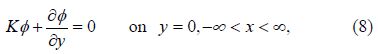
If the upper surface of the ocean is a free surface, then the linearised boundary condition is given by

where, $~K=\frac{{{\sigma }^{2}}}{g},g$is the acceleration due to gravity. In this case, $l={{\nu }_{0}}\text{sin}\alpha ,$where ${{\nu }_{0}}$ is given by the unique positive real root of the dispersion equation: $$\nu \text{sinh}\nu h-K\text{cosh}\nu h=0$$

The symmetric and anti-symmetric multipoles are constructed as

where, $A\left( \mu \right),{{A}_{1}}\left( \mu \right),B\left( \mu \right)$ and ${{B}_{1}}\left( \mu \right)$ are functions of to be determined. Now, by utilising the boundary condition(2) and (8), we obtain $$\begin{align} & ~~A\left( \mu \right)=\frac{{{(-1)}^{n+1}}{{\text{e}}^{-\nu \left( h-f \right)}}\text{cosh}n\mu }{\text{cosh}\nu h} \\ & ~~~B\left( \mu \right)=\frac{\text{cosh}n\mu \left( \text{cosh}\nu h\left( \nu +K \right){{\text{e}}^{-\nu f}} \right)-\left( {{(-1)}^{n}}\nu {{\text{e}}^{-\nu \left( h-f \right)}} \right)}{\text{cosh}\nu h\left( \nu \text{sinh}\nu h-K\text{cosh}\nu h \right)} \\ \end{align}$$ Thus, for the case of symmetric multipoles, using(9), we obtain where, $$\begin{align} & F_{n}^{1s}\left( \nu ,y \right)=\left( K\text{sinh}\nu y-\nu \text{cosh}\nu y \right){{\text{e}}^{-\nu \left( h-f \right)}}+ \\ & {{(-1)}^{n}}\text{cosh}\nu \left( h-y \right)\left( \nu +K \right){{\text{e}}^{-\nu f}} \\ \end{align}$$

The contour of the integration in(11)is indented below the pole at $\mu ={{\mu }_{0}}=\text{cos}{{\text{h}}^{-1}}\frac{{{\nu }_{0}}}{l}$ on the real $\mu $ axis to take care of the outgoing nature of the wave as $\left| x \right|\to \infty $ .The far-field form of the multipoles is obtained as

where, $$\beta =\sqrt{\nu _{0}^{2}-{{l}^{2}}},N_{0}^{2}=\frac{2{{\nu }_{0}}h}{2{{\nu }_{0}}h+\text{sinh}2{{\nu }_{0}}h}$$ and

From(13), it is observed that

${{a}_{n+1}}+\frac{\text{cosh}\left( n+1 \right){{\mu }_{0}}}{\text{cosh}n{{\mu }_{0}}}\text{tanh}{{\nu }_{0}}\left( h-f \right){{a}_{n}}=0\text{ }\!\!~\!\!\text{ }$ when n is even, and ${{a}_{n+1}}+\frac{\text{cosh}\left( n+1 \right){{\mu }_{0}}}{\text{cosh}n{{\mu }_{0}}}\text{coth}{{\nu }_{0}}\left( h-f \right){{a}_{n}}=0\text{ }\!\!~\!\!\text{ }$ when n is odd.

Therefore, the following linear combinations of the multipoles $\phi _{n+1}^{s}+\frac{\text{cosh}\left( n+1 \right){{\mu }_{0}}}{\text{cosh}n{{\mu }_{0}}}\text{tanh}{{\nu }_{0}}\left( h-f \right)\phi _{n}^{s}\text{ }\!\!~\!\!\text{ }$ when is even, and $\phi _{n+1}^{s}+\frac{\text{cosh}\left( n+1 \right){{\mu }_{0}}}{\text{cosh}n{{\mu }_{0}}}\text{coth}{{\nu }_{0}}\left( h-f \right)\phi _{n}^{s}\text{ }\!\!~\!\!\text{ }$ when is odd, do not contribute anything as $\left| x \right|\to \infty $ so that they are wave-free. The oblique symmetric wave-free potentials having singularity at (0,f) are constructed in this case as

when n is even, and when n is odd. By a similar procedure the oblique anti-symmetric wave-free potentials can be obtained, by utilising(10), as when n is even, when n is odd and $$F_{n}^{1a}\left( \nu ,y \right)=\left( K\text{sinh}\nu y-\nu \text{cosh}\nu y \right){{\text{e}}^{-\nu \left( h-f \right)}}-{{(-1)}^{n}}\text{cosh}\nu \left( h-y \right)\left( \nu +K \right){{\text{e}}^{-\nu f}}$$

If $l\to 0$ the limiting forms of the wave-free potentials are given by

when n is even, and when n is odd and the anti-symmetric wave-free potentials are when n is even, when n is odd. These forms were obtained by Linton and McIver(2001)in case of two dimensional motion in finite depth water.

If the singularity is situated at the upper surface of water, then the wave-free potentials can be obtained from(14)-(17)by making $f\to 0$ and they are given by

when n is even, and when n is odd. For the anti-symmetric wave-free potentials, when n is even, when n is odd. Here, $$F_{n}^{01s}\left( \nu ,y \right)=\left( K\text{sinh}\nu y-\nu \text{cosh}\nu y \right){{\text{e}}^{-\nu h}}+{{(-1)}^{n}}\text{cosh}\nu \left( h-y \right)\left( \nu +K \right)$$ and $$F_{n}^{01a}\left( \nu ,y \right)=\left( K\text{sinh}\nu y-\nu \text{cosh}\nu y \right){{\text{e}}^{-\nu h}}-{{(-1)}^{n}}\text{cosh}\nu \left( h-y \right)\left( \nu +K \right)$$

3.2 Effect of surface tension at the upper surface

If the effect of surface tension is included at the free surface, then the linearised free surface condition is given by on

where, $M=\frac{T}{\rho g}$,T is the coefficient of surface tension at the free surface and $\rho $ is the density of water. In this case, $l={{\kappa }_{0}}\text{sin}\alpha $, where ${{\kappa }_{0}}$ is the unique positive real root of the dispersion equation $\kappa \left( 1+M{{\kappa }^{2}} \right)\text{sinh}\kappa h-K\text{cosh}\kappa h=0$

Proceeding as before, the symmetric multipoles can be constructed as

where $$F_{n}^{2s}\left( \nu ,y \right)=\left( K\text{sinh}\nu y-\nu \left( 1+M{{\nu }^{2}} \right)\text{cosh}\nu y \right){{\text{e}}^{-\nu \left( h-f \right)}}+{{(-1)}^{n}}\text{cosh}\nu \left( h-y \right)\left( \nu \left( 1+M{{\nu }^{2}} \right)+K \right){{\text{e}}^{-\nu f}}$$ and the contour of the integration in(27)is indented below the pole at $\mu ={{\mu }_{1}}=\text{cos}{{\text{h}}^{-1}}\frac{{{\kappa }_{0}}}{l}$ . It is easy to see that $\phi _{n+1}^{s}+\frac{\text{cosh}\left( n+1 \right){{\mu }_{1}}}{\text{cosh}n{{\mu }_{1}}}\text{tanh}{{\kappa }_{0}}\left( h-f \right)\phi _{n}^{s}\text{ }\!\!~\!\!\text{ }$ when n is even and $\phi _{n+1}^{s}+\frac{\text{cosh}\left( n+1 \right){{\mu }_{1}}}{\text{cosh}n{{\mu }_{1}}}\text{coth}{{\kappa }_{0}}\left( h-f \right)\phi _{n}^{s}\text{ }\!\!~\!\!\text{ }$ when n is odd, do not contribute anything as $\left| x \right|\to \infty $ o that they are wave-free. In this case, the oblique symmetric wave-free potentials having singularity at are (0,f) constructed as when n is even and when n is odd. Similarly, the oblique anti-symmetric wave-free potentials are obtained as when is even, when n is odd. Here $$F_{n}^{2a}\left( \nu ,y \right)=\left( K\text{sinh}\nu y-\nu \left( 1+M{{\nu }^{2}} \right)\text{cosh}\nu y \right){{\text{e}}^{-\nu \left( h-f \right)}}-{{(-1)}^{n}}\text{cosh}\nu \left( h-y \right)\left( \nu \left( 1+M{{\nu }^{2}} \right)+K \right){{\text{e}}^{-\nu f}}$$

As before, if $l\to 0$ the limiting forms of the wave-free potentials are given by

when n is even and when n is odd. Similarly the anti-symmetric wave-free potentials become as $l\to 0$ when n is even and when n is odd.

Making $f\to 0$ the free surface oblique wave-free potentials are obtained from(28)-(31)as

when n is even and when n is odd. The oblique anti-symmetric wave-free potentials are when n is even and when n is odd. Here, $$F_{n}^{02s}\left( \nu ,y \right)=\left( K\text{sinh}\nu y-\nu \left( 1+M{{\nu }^{2}} \right)\text{cosh}\nu y \right){{\text{e}}^{-\nu h}}+{{(-1)}^{n}}\text{cosh}\nu \left( h-y \right)\left( \nu \left( 1+M{{\nu }^{2}} \right)+K \right)$$ and $$F_{n}^{02a}\left( \nu ,y \right)=\left( K\text{sinh}\nu y-\nu \left( 1+M{{\nu }^{2}} \right)\text{cosh}\nu y \right){{\text{e}}^{-\nu h}}-{{(-1)}^{n}}\text{cosh}\nu \left( h-y \right)\left( \nu \left( 1+M{{\nu }^{2}} \right)+K \right)$$

3.3 Water with an ice cover

If the upper surface of the ocean is covered by an ice-cover modelled as a thin elastic plate, then the boundary condition at the upper surface is given by

where $D=\frac{Eh_{0}^{3}}{12\left( 1-{{\tau }^{2}} \right)g\rho },$ E and $\tau $ being the Young’s modulus and Poisson’s ratio of the elastic plate. $\varepsilon =\frac{{{\rho }_{0}}{{h}_{0}}}{\rho },$ being the small thickness of the ice-cover and is the density of ice. Here $l={{\lambda }_{0}}\text{sin}\alpha ,$ being the unique positive real root of the dispersion equation $\lambda \left( 1+D{{\lambda }^{4}}-\varepsilon K \right)\text{sinh}\lambda h-K\text{cosh}\lambda h=0.$

In this case, the symmetric multipoles are constructed as

where $$F_{n}^{3s}\left( \nu ,y \right)=\left( K\text{sinh}\nu y-\nu \left( 1+D{{\nu }^{4}}-\varepsilon K \right)\text{cosh}\nu y \right){{\text{e}}^{-\nu \left( h-f \right)}}+{{(-1)}^{n}}\text{cosh}\nu \left( h-y \right)\left( \nu \left( 1+D{{\nu }^{4}}-\varepsilon K \right)+K \right){{\text{e}}^{-\nu f}}$$ and the contour of the integral in(41)is indented below the pole at $\mu ={{\mu }_{2}}=\text{cos}{{\text{h}}^{-1}}\frac{{{\lambda }_{0}}}{l}.$ It can be shown that the combination of the multipoles $$\phi _{n+1}^{s}+\frac{\text{cosh}\left( n+1 \right){{\mu }_{2}}}{\text{cosh}n{{\mu }_{2}}}\text{tanh}{{\lambda }_{0}}\left( h-f \right)\phi _{n}^{s}\text{ }\!\!~\!\!\text{ }$$ when n is even and $$\phi _{n+1}^{s}+\frac{\text{cosh}\left( n+1 \right){{\mu }_{2}}}{\text{cosh}n{{\mu }_{2}}}\text{coth}{{\lambda }_{0}}\left( h-f \right)\phi _{n}^{s}\text{ }\!\!~\!\!\text{ }\!\!~\!\!\text{ }$$ when n is odd do not contribute anything as $\left| x \right|\to \infty $ so that they are wave-free. The oblique symmetric wave-free potentials are constructed as when n is even, when n is odd and the path of integration(42) and (43)is indented below the pole at $\mu ={{\mu }_{2}}=\text{cos}{{\text{h}}^{-1}}\frac{{{\lambda }_{0}}}{l}.$ By a similar procedure as above, the anti-symmetric oblique wave-free potentials are obtained as when n is even, when n is odd and $$F_{n}^{3a}\left( \nu ,y \right)=\left( K\text{sinh}\nu y-\nu \left( 1+D{{\nu }^{4}}-\varepsilon K \right)\text{cosh}\nu y \right){{\text{e}}^{-\nu \left( h-f \right)}}-{{(-1)}^{n}}\text{cosh}\nu \left( h-y \right)\left( \nu \left( 1+D{{\nu }^{4}}-\varepsilon K \right)+K \right){{\text{e}}^{-\nu f}}$$

As before, if $l\to 0$ the limiting forms of the wave-free potentials are given by

when n is even and when n is odd. Similarly the anti-symmetric wave-free potentials become as $l\to 0$ when n is even and when n is odd. Making $f\to 0$ the free surface oblique wave-free potentials are obtained from(41)-(45)as when n is even and when n is odd. Similarly, the oblique anti-symmetric wave-free potentials are when n is even, when n is odd. Here $$F_{n}^{03s}\left( \nu ,y \right)=\left( K\text{sinh}\nu y-\nu \left( 1+D{{\nu }^{4}}-\varepsilon K \right)\text{cosh}\nu y \right){{\text{e}}^{-\nu h}}+{{(-1)}^{n}}\text{cosh}\nu \left( h-y \right)\left( \nu \left( 1+D{{\nu }^{4}}-\varepsilon K \right)+K \right)$$ and $$F_{n}^{03a}\left( \nu ,y \right)=\left( K\text{sinh}\nu y-\nu \left( 1+D{{\nu }^{4}}-\varepsilon K \right)\text{cosh}\nu y \right){{\text{e}}^{-\nu h}}-{{(-1)}^{n}}\text{cosh}\nu \left( h-y \right)\left( \nu \left( 1+D{{\nu }^{4}}-\varepsilon K \right)+K \right)$$

4 Numerical results

The velocity potential $\Phi \left( x,y,z,t \right)$ describing the wave motion corresponding to the wave-free potential ${{\Psi }_{n}}\left( x,y,z,t \right)$ can be written as

Now, we write $$\Phi \left( x,y,z,t \right)=\text{Re}\left[ \phi \left( x,y \right){{\text{e}}^{-\text{i}\left( \sigma t+lz \right)}} \right]$$ and $${{\Psi }_{n}}\left( x,y,z,t \right)=\text{Re}\left[ {{\psi }_{n}}\left( x,y \right){{\text{e}}^{-\text{i}\left( \sigma t+lz \right)}} \right]$$ so that the non-dimensional form of the depression of the upper surface of water is $$\chi \left( x,z,t \right)=\frac{1}{f}\frac{1}{g}\frac{\partial \Phi \left( x,0,z,t \right)}{\partial t}=-\text{Re}\left[ \text{i}{{\psi }_{n}}\left( x,0 \right){{\text{e}}^{-\text{i}\left( \sigma t+lz \right)}} \right]$$

Writing $$\chi \left( x,z,t \right)=\text{Re}\left[ \xi \left( x,t \right){{\text{e}}^{-\text{i}lz}} \right]$$ we find

For numerical computation we choose $\sigma t=\frac{\text{ }\!\!\pi\!\!\text{ }}{2}$, then

are the non-dimensional forms of the depression of the upper surface for symmetric and anti-symmetric wave-free potentials respectively. The profile $\xi $ of the upper surface of water is plotted against the non-dimensional spatial variable $\left( x'=\frac{x}{f} \right)$ in a number of figures by utilising(56) and the forms of the wave-free potentials $\psi _{n}^{s,a}\left( x,y \right)$ is given by(14)to(17)for the case of free surface, (36)to(39)for the case of free surface with surface tension, and (42)to(45)for the case of ice-cover modelled as a thin elastic plate.

For different values of corresponding to the angle of incidence $\alpha =0,\frac{\text{ }\!\!\pi\!\!\text{ }}{6},\frac{\text{ }\!\!\pi\!\!\text{ }}{4}(lf=0,0.2703,0.382),$ the depression of the free surface ${{\xi }^{s}}$ and ${{\xi }^{s}}$ are plotted in Fig.3 and Fig.4 by taking Kf=0.5, h/f=3 and n=2. In Fig.5 and Fig.6, ${{\xi }^{s}}$ and ${{\xi }^{a}}$ are depicted taking n=2, 5 respectively where other parameters remains same as in Fig.1 and Fig.2. In all these cases, it is observed that the amplitudes of oscillations of ${{\xi }^{s,a}}$ of both symmetric and anti-symmetric wave-free potentials diminish as increases and ultimately tend to zero, which is expected since $\psi _{n}^{s,a}\left( x,y \right)$ tends to zero always far from the point of singularity.

When the effect of surface tension is included at the free surface, ${{\xi }^{s,a}}$ are depicted graphically in Fig.7 to Fig.10 against ${x}'.$ In the Fig.7 and Fig.8 , ${{\xi }^{s}}$ and ${{\xi }^{a}}$ are plotted against ${x}'$ respectively for different values of ${M}'=\frac{M}{{{f}^{2}}}=1,0.1,0.001$ when the angle of incidence is chosen as $\alpha =\frac{\text{ }\!\!\pi\!\!\text{ }}{4}$ and $Kf=0.5,n=2,h/f=3.$

Here, the amplitudes of are seen to decrease due to the effect of the surface tension at the upper surface. For a sufficiently small value of ${M}'=0.001$, the profiles of ${{\xi }^{s,a}}$, a are similar to those in Fig.1 and Fig.2.

For a fixed value of ${M}'=0.1,$ ${{\xi }^{s}}$ for n=2 is depicted in Fig.9 for different values of corresponding to $\alpha =0,\frac{\text{ }\!\!\pi\!\!\text{ }}{6},\frac{\text{ }\!\!\pi\!\!\text{ }}{4},\left( lf=0,0.2644,0.3733 \right)$ and in Fig.10, ${M}'=0.1,$ ${{\xi }^{s}}$ is plotted for different values of Kf=0.5, 0.8, 1.0 and $\alpha =\frac{\text{ }\!\!\pi\!\!\text{ }}{4}\left( lf=0.3733 \right)$ by taking h/f=3. It is observed from Fig.10 that the maximum amplitude of decreases as kf increases.

If the upper surface of water is covered by an ice sheet modelled as a thin elastic plate, the depression ${{\xi }^{s,a}}$ of the upper surface is depicted graphically against ${x}'$ in Fig.11 to Fig.14. In Fig.11 and Fig.12, ${{\xi }^{s,a}}$ for n=2 are plotted for different values of the non-dimensional stiffness parameter ${D}'=\frac{D}{{{f}^{4}}}$ =0.001, 0.1, 1 and mass parameter ${\varepsilon }'=\frac{\varepsilon }{f}$ =0.01 while the angle of incidence is taken as $\alpha =\frac{\text{ }\!\!\pi\!\!\text{ }}{4}$ and $Kf=0.5,h/f=3.$ It is observed from these figures that the amplitudes of ${{\xi }^{s,a}}$ decrease due to the presence of the elastic ice-cover at the upper surface of water. For a sufficiently small value of ${D}'=0.001$ the profiles of ${{\xi }^{s,a}}$ almost coincide with those in Fig.1 and Fig.2 for the case of free surface while all other parameters remain the same.

For fixed values of ${D}'=0.1,{\varepsilon }'=0.01,$ ${{\xi }^{s}}$is depicted in Fig.13 for different values of Kf = 0.5, 0.8, 1.0 when $\alpha =\frac{\text{ }\!\!\pi\!\!\text{ }}{4},\left( lf=0.4823 \right)$ and h/f = 3 and n = 2 respectively. Like previous cases, here also the amplitude of ${{\xi }^{s}} is observed to decrease with the increase of Kf. However, in Fig.14, is plotted for different values of lf corresponding to $\alpha =0,\frac{\text{ }\!\!\pi\!\!\text{ }}{6},\frac{\text{ }\!\!\pi\!\!\text{ }}{\text{4}},\left( lf=0,0.3948,0.4823 \right)$ by taking Kf = 0.5, h/f=3, n=2.

5 Conclusions

In the linearised theory of water waves wave-free potentials have been derived in the literature by using multipole expansion of the potential function for finite or infinitely deep water with a free surface. Taking the effect of surface tension into account or for water with an ice-cover, the expressions of the oblique wave-free potentials having singularity at a point submerged in water of uniform finite depth are constructed here in a systematic manner by taking appropriate linear combinations of the multipoles. These wave-free potentials decay as one moves away from the point of singularity. The depression of the upper surface related to these wave-free potentials is depicted graphically for each case in a number of figures. In each figure, it is observed that the wave profile of the depression of the upper surface rapidly diminishes with the distance from the origin which is plausible since the wave-free potentials decay rapidly from the point of singularity. These figures also show that the coefficient of surface tension and the stiffness parameter of the elastic ice-cover affect the resulting wave motion. The results for non-oblique wave-free potentials are derived by making $l\to 0$ i. e $\alpha =0$ and the upper surface wave-free potentials are obtained by making $f\to 0$ The limiting case $l\to 0$ for non-oblique wave-free potentials in finite depth water with a free surface coincide with those given by Linton and McIver(2001).

The wave-free potentials constructed here will be useful in the mathematical study of water wave problems involving infinitely long horizontal cylinders, either half-immersed or completely submerged are used in the construction of offshore structures for extraction of crude oil deposited below the ocean floor. Further extension of the above results can be made by considering generalised boundary condition involving higher order derivatives at the upper surface of water.Acknowledgement

The authors thank to the Reviewer for his valuable comments and suggestions to revise the paper.