1 Introduction

The marine diesel engine is a very complicated mechanical system. These engines offer various advantages such as high efficiency, high power concentration and long operational life time. In recent years, the main aim in internal combustion engine development has been the reduction of emissions, in order to satisfy ever stricter emission regulations while maintaining similar levels of efficiency, power density, reliability and lifecycle cost. On the other h and , their large size can cause great difficulties in the diagnosis of improper operation. A promising way to enhance optimization and diagnosis systems is to adopt fast and accurate model-based techniques that minimize the requirement for costly test-bed measurements for this multi-variable optimization.

In this paper, the overall engine system is divided into several functional blocks: cooling, lubrication, air, injection, combustion, and emissions.

Engine cooling system plays an important role to maintain the operating temperature of engine. The coolant circuit initiates by picking up heat at water jackets. Several control, design and diagnostic oriented models for the cooling systems have been developed. Dynamic models based on thermal modeling are developed for thermal management systems(Salah et al., 2010) and for the diagnosis of diesel engine(Yoo et al., 2000). The model developed by De Persis and Kallesøe(2008; 2009a)is based on network theory and the well known analogy between electrical and hydraulic circuits. Based on these works, a dynamic model for the cooling system of the diesel engine was developed.

The oil system reduces friction by creating a thin film between moving parts, which helps form a gastight seal between piston rings and cylinder walls. Haas et al.(1991)studied the influence of oil parameters on the engine operating pumps, Chun(2003)gives the mathematical model for oil flow through a hydraulic tappet as well as those of an oil jet and plain journal bearing, calculate the distribution of flow and pressure of the lubrication system. Based on these models a lubrication model has been reformed.

The fuel-injection system is responsible for supplying the diesel engine with fuel. The common rail injection system improves engine performance, noise and emissions are reduced(Stumpp and Ricco, 1996). Gupta et al.(2011)develop a one-dimensional distributed model for the common rail by using basic fluid flow equations, which can capture the distributed dynamics of the pressure disturbances in the rail. In this work, the developed model(Lino et al., 2007)representing the injection system in details in a reliable replication of reality has been adopted.

The purpose of the air-path is to convey and control the gases used during the normal diesel engine operative condition. The behavior of the various components of the system is described based on known physical laws(Heywood, 1988)as the laws of conservation of mass and energy and the first law of dynamics. Zito and Landau(2005)present a nonlinear system identification procedure based on a polynomial NARMAX representation and is applied to a variable geometry turbocharged diesel engine. Karlsson et al.(2010)presents an identification procedure by identifying local linear models at each operating point. Among the various known physical models(quasi-static, drain/filling, bond graph…), the quasi-static model mean values(Younes, 1993; Omran et al., 2008)has been adopted due to its simplicity and accuracy in describing the behavior of the different components. We seek simplicity as these models are designed in order to be used in a heavy dynamic optimization process.

The exhaust gases that are discharged from the engine contains CO, NO_x, PM, HC, Soot and CO₂. Hiroyasu et al., (1983)present a semi empirical model to predict the emissions. Chemical equations that describe the formation of these compounds were studied by Heywood(1988), Ferguson and Kirkpatrick(2001), Lipkea and DeJoode(1994), Mansouri and Bakhshan(2001), and Hiroyasu et al.(1983). Based on these works an emission model has been developed.

For thermodynamic cycle ideal models provide the simplest way to reproduce internal combustion engine(ICE)cycles, but they usually do not represent with sufficient accuracy the actual behavior of an ICE. The most recent study(Sakhrieh et al., 2010)presents a diesel engine simulation where a dual Wiebe function(Wiebe, 1956)was used to model the heat release while the convective heat transfer coefficient is given by the Woschni model(Woschni, 1967). In this paper, the thermodynamic cycle used is the one developed by Basbous et al.(2012)that takes into account the heat transfer to the chamber walls, the fuel injection, the instantaneous change in gas properties, the kinematic model of gas volume, the specific sub-models for the calculation of the energy and mass equations terms.

Many diesel engine simulators have been developed. DiSim V1.0 is a diesel simulator of RTZ-Soft society, the simulator calculates the thermodynamic and gas dynamic of internal combustion engines. ASM from Dspace society is a mean value engine model with crank-angle-based torque generation, dynamic manifold pressure, temperature calculation, and several fuel injection models. These simulators and others(AVL Boost, DNV GL COSMOSS and Mother)are simulation programs, which can output many parameters for the combustion process. The air system, emissions without incorporating the lubrication, injection and cooling system that influence the performance of diesel engines are not independent, but influence each other.

From this reason, it is impossible to predict the engine performance precisely if the simulator calculates, for example, the combustion when cylinder wall temperature is constant. Other simulators, such as GT-Power, present a modeling of all subsystems, but use some black box models(Neural networks are used in mean-value cylinders to speed up the calculations). In addition, for diesel engine GT-Power simulate the emissions only of No_x and Soot.

In this work, a complete simulator for diesel engine incorporating several functional blocks: cooling, lubrication, air, injection, combustion, and emissions has been developed. The dynamics of the overall engine system are expressed as a set of simultaneous algebraic and differential equations.

This paper is organized as follows. In sections 2.1 to 2.7, a simulator model of a marine diesel engine based on physical, semi-physical, mathematical and thermodynamic equations is presented. A deep description and analysis of the functioning in addition to exhibition of the simulations that were carried out to validate the following sub-blocks: cooling, lubrication, injection, air system, combustion, and gas emissions. The conclusion is given in section 3.

2 Systems of the marine diesel engine

The different subsystems of marine diesel engine are: cooling, lubrication, air, injection, combustion and emissions, as shown in Fig. 1. Dynamic characteristics of each subsystem are expressed in mathematical equations, and the overall engine system dynamics is thus expressed as a set of simultaneous algebraic and differential equations. The dynamics of each sub-block of the marine engine have been validated by experimental results.

The test bench used in this work is a marine diesel engine manufactured by the company SIMB under the reference 6M26SRP1(Fig. 2). The engine has six-cylinders with direct injection, a power ranging up to 331 kW, a maximum speed of 1 800 r/min.

The main characteristics of the engine are summarized in Table 1. The characteristics of different subsystems of the test bench are as below:

1)Engine and block: cast iron cylinder block, one inspection door per cylinder for access to conrod cap, cast iron cylinder liners, separate cast iron cylinder heads equipped with 4 valves replaceable valves guides and seats, hardened steel forged crankshaft with induction hardened journals, camshaft with polynomial cams profile, distribution with tempered, hardened and grinded helicoïdal gears, chromium-Molibdenum steel conrods, lube oil cooled light alloy pistons with high performance, piston rings.

2)Cooling system: fresh/raw water heat exchanger with integrated thermostatic valves and expansion tank, cast iron centrifugal fresh water pump mechanically driven, bronze self priming raw water pump mechanically driven.

3)Lubrication system: full flow screwable oil filters, lube oil purifier with replaceable cartridge, fresh water cooled lube oil cooler.

4)Fuel system: in line injection pump with flanged mechanical governor, double wall injection bundle with leakage collector, duplex fuel filters replaceable engine running.

5)Air system: fresh water cooled turbo blower, double flow raw water cooled intake air cooler.

The engine is connected to a system controller for speed and torque control. The different sensors used on the test bench are presented in Table 2.

2.1 Cooling system 2.1.1 Description

Engine cooling system plays an important role to maintain the operating temperature of engine. The coolant circuit initiates by picking up heat at water jackets. The cooling system consists of two circuits: a sea water circuit and fresh water circuit. Each circuit is activated with a pump, depending on the temperature of the fresh water, a thermostat control the flow of water to the heat exchanger when it is hot, or directly to the pump if it is relatively cold. The system cools also the oil before its inlet to the engine, and cools the air going to combustion chamber at its outlet from the compressor. The components of the system, shown in Fig. 3 are similar to the one of the test bench, the sea water are replaced by water from a tank.

2.1.2 Model of cooling system

The following equations represent the modeling of cooling system(Paradis et al., 2002; Heywood, 1988): the temperature model is based on Newton’s cooling law, the pressure pump model is based on Bernoulli equation for the incompressible fluids.

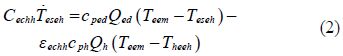
Engine block outlet:

where C_B is the engine block capacity, Q_ed is the flow pump fresh water, c_ped is the fresh water specific heat, T_esm is the fresh water temperature at the engine outlet, T_eseh is the water temperature at oil heat exchanger outlet, is the fuel flow, A_p is the piston internal surface, b₁ and b₂ are constants determined experimentally.

Oil-water heat exchanger outlet:

where c_echh is the oil heat exchanger capacity, Q_h is the flow of oil, c_ph is the oil specific heat, T_eem and T_heeh are the water and oil temperature at oil heat exchanger inlet, respectively.

Air-water heat exchanger outlet:

where C_echa is the air heat exchanger capacity, Q_a is the flow of air, c_pa is the air specific heat, T_esea and T_asc are the water temperature at the air heat exchanger outlet and air temperature at compressor outlet, respectively, k_a is constant in normal operation(between 0 and 1), depends to the ratio of water going to the air-water heat exchanger.

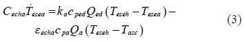
Water heat exchanger outlet(sea water):

where C_eche is the water heat exchanger capacity, T_ebts the sea water temperature at the heat exchanger outlet, and K_th the opening of the linear opening of the thermostat between 77 °C and 87 °C. Q_ebt, ε_eche, c_pebt, T_ebte are the pump sea water flow, heat exchanger efficiency, calorific capacity of the sea water, sea water temperature at the heat exchanger outlet, respectively.

Outlet pump fresh water(De Persis and Kallesøe, 2009b):

where P_eem and P_eep are respectivly the outlet and inlet pressure of the fresh water pump. W is the crankshaft rotational speed, R_deq is the equivalance resistance of the fresh water circuit. K₁, K₂ are constants in normal operation, depends on the water density, viscosity and to the ratio(pump gear diameter/crankshaft gear diameter)in relation. The same modeling is used at the outlet of the pump sea water.

2.1.3 Experimental validation

The cooling system model in normal operation has been validated by comparing the measured outputs of the real system with the estimated outputs simulated under Matlab/Simulink, which demonstrated the effectiveness of the proposed model. Fig. 4 represent measured values of crankshaft rotation speed(W) and the torque(T)that comm and the engine, also, the measured and estimated values respectively of the water temperature at the outlet of the engine block, the sea water temperature at the heat exchanger outlet and the freshwater pump pressure.

2.2 Lubrication system 2.2.1 Description

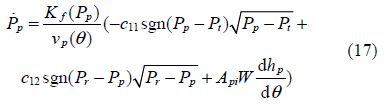
Engine oil performs several basic functions in order to provide adequate lubrication. It works to keep the engine clean and free from rust and corrosion. Engine oil is expected to provide a protective film, to prevent metal to metal contact(wear) and reduce friction. It must help remove heat from engine surfaces, and flush away wear particles. It also aids in sealing the piston rings, serves as a hydraulic fluid. The lubrication circuit of combustion engine involves many components(Fig. 5). This circuit is supplied with oil via a volumetric pump. With this type of pump, the oil pressure depends on rotational speed as well as the viscosity of typical oil. To avoid oil system deterioration problems caused by pressure, it is necessary to provide pump with a pressure relief valve(discharge valve). The impurities, that could alter the functioning parts, are suspended in typical oil and are filtered out. Typical oil is then distributed to the various components subject to friction(piston, camshaft)before descending down into the housing.

2.2.2 Model of lubrication system

The different components of the system are modeled as below:

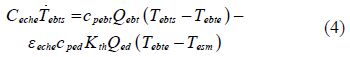
Block engine outlet:

where T_hsm, T_hem are oil temperature at the outlet and inlet of the block engine, respectively.

Oil-Water heat exchanger outlet:

where T_hse is the oil temperature at oil heat exchanger outlet.

Pressure outlet filter:

where P_hsf, P_hef are filter outlet and inlet pressure, respectively. K_hf is constant in normal operation depends to the filter caracteristics.

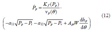
Oil pump outlet:

The same modeling of fresh water pump is used. In this case, K₃ and K₄ the substitute of K₁ and K₂ are not constant, they are directly proportional of the oil density and oil kinematics viscosity expressed as:

where T₀ is the ambient temperature, ρ₀ is the oil density at T₀.

2.2.3 Experimental validation

The model of the lubrication system is validated by comparing the outputs of the real system(using the test bench)to the outputs estimated by the model. Fig. 6 represent measured values of crankshaft rotation speed(W) and the torque(T)that comm and the engine, and respectively the measured oil temperature at the outlet of the engine block, the oil pressure at the outlet of the pump, the oil pressure at the outlet of the filter and the corresponding estimated values.

2.3 Injection system 2.3.1 Description

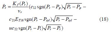
The injection system drives fuel from tank to combustion chamber. The main elements of a common rail diesel injection system are: a low pressure circuit, including the fuel tank and a low pressure pump, a high pressure pump with a delivery valve, a common rail and the electro injectors. The low pressure pump sends the fuel coming from the tank to the high pressure pump. Hence the pump pressure raises, and when it exceeds a given threshold, the delivery valve opens, allowing the fuel to reach the common rail, which supplies the electro-injectors. The common rail hosts an electro-hydraulic valve driven by the electronic control unit(ECU), which drains the amount of fuel necessary to set the fuel pressure to a reference value. The valve driving signal is a square current with a variable duty cycle(i.e. the ratio between the length of on and the off phases), which in fact makes the valve to be partially opened and regulates the rail pressure. The high pressure pump is of reciprocating type with a radial piston driven by the eccentric profile of a camshaft. It is connected by a small orifice to the low pressure circuit and by a delivery valve with a conical seat to the high pressure circuit. When the piston of the pump is at the lower dead centre, the intake orifice is open, and allows the fuel to fill the cylinder, while the downstream delivery valve is closed by the forces acting on it. Then, the closure of the intake orifice, due to the camshaft rotation, leads to the compression of the fuel inside the pump chamber. When the resultant of valve and pump pressures overcomes a threshold fixed by the spring preload and its stiffness, the shutter of the delivery valve opens and the fuel flows from the pump to the delivery valve and then to the common rail. As the flow sustained by the high pressure pump is discontinuous, a pressure drop occurs in the rail due to injections when no intake flow is sustained, while the pressure rises when the delivery valve is open and injectors closed. Thus, to reduce the rail pressure oscillations, the regulator acts only during a specific camshaft angular interval(activation window in the following), and its action is synchronized with the pump motion. The main elements of an electro-injector for diesel engines are a control chamber and a distributor. The former is connected to the rail and to a low pressure volume, where both inlet and outlet sections are regulated by an electro-hydraulic valve. During normal operations the valve electro-magnetic circuit is off and the control chamber is fed by the high pressure fuel coming from the common rail. When the electro-magnet circuit is excited, the control chamber intake orifice closes while the outtake orifice opens and so a pressure drop occurs. When the injection orifices open, the cylinders receive the fuel. The energizing time depends on the fuel amount to be injected. The system is presented in the Fig. 7(Lino et al., 2007).

2.3.2 Model of injection system

The different components of the system are modeled as:

where P_p, P_v, P_r, P_i, P_cyl are the pressure pump, delivery valve, rail, injector, and the pressure inside cylindre, respectively. K_f is related to the fuel pressure in every components(Heywood, 1988). v_p(θ)is pump chamber volume function of θ(crankshaft angle). v_v, v_r, v_i are respectivly the delivery valve volume, rail volume, injector volume. A_pi is the cylinder bore, h_p is the piston instantaneous axial displacement of the pump. E_T is a square signal equal to 1 during injections. a_ij are positive constant parameters in normal operation, depends to the fuel density and output flow sections(Lino et al., 2007). u is an electronic signal to control the flow from the rail to the tank, c_{d, cyl} is the disharge coefficient.

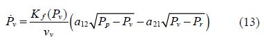
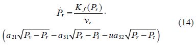
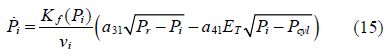
The model order is reduced by neglecting the delivery valve and injection pressures dynamics. This is tantamount to consider, for each time instant, the flow between the pump and the delivery valve equal to the flow between the delivery valve and the rail; and the flow between the rail and the injectors equal to the flow between the injectors and cylinders. With this simplification, the system state equations become :

where E_T16 is the sum of 6 electronics signal to control the opening of the 6 injectors, c_ij are positive constants(Lino et al., 2007).

2.3.3 Experimental validation

The eccentric profile of the camshaft that drives the reciprocating type high pressure pump creates the periodic pressure pulse in the pump as shown in Fig. 8. At certain threshold the delivery valve open and rise the common rail pressure, the electrodynamic valve driven by the ECU, control the common rail pressure to a reference value by draining the excess fuel back to the tank. When the electromagnet circuit of the injector is excited, the common rail, feeding the control chamber, pressure will drop as shown in Fig. 8. Fig. 9 shows that as the fuel rate increases the torque developed by the engine increases as well as the engine speed.

2.4 Air system 2.4.1 Description

The air systemworks described by Younes(1993) and Omran et al.(2008)has been adopted in the model since it accurately describes the air system behavior of the motor in a relatively simple manner. the state variables are represented by their average values eliminating any dependency on the angular position of the crankshaft. The engine system as described in Fig. 10 comprises five blocks(intake manifold, exhaust manifold, heat exchanger, the engine variable geometry turbocharger). Detailed description of the system is presented in Omran et al.(2008; 2009).

2.4.2 Model of air system

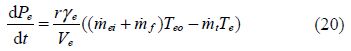
The global model of the engine air system is described by the six differential equations, describing the five blocks.

1)Pressure at intake manifold:

where r is the constant of prefect gas relative to air, γ_a is the ratio of thermal capacity at constant pressure and air volume. P_a, V_a and T_a are the air pressure, volume and temperature in the intake maniflod. T_{c, ech} is the air temperature at the air heat exchanger outlet. are respectivly the air flow at compressor outlet and cylinder inlet.

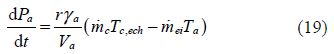
2)Pressure at exshaust manifold:

3)Air flow mass at intake manifold:

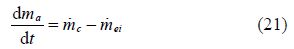
4)Air flow mass at esxhaust manifold:

where m_t is the air flow at turbine inlet.

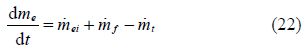
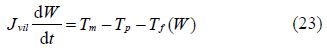
5)Crankshaft rotation(Fossen, 2002):

where J_vil is the crankshaft inertia, T_m is the motor torque, T_p is the propeller, T_f(W) is the friction torque.

6)Turbocompressor rotation:

where w_tc, I_tc are the angular velocity and turbocompressor inertia., and are the mecanichal, compressor and turbine efficiency. C_pe, C_pa are the exhaust and intake manifold air calorific capacity. T₀ is the air temperature at compressor inlet., are the compression and detente ratio.

2.4.3 Experimental validation

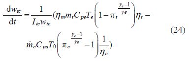
Fig. 11 represent measured values of the torque(T)that comm and the engine, compare the measured and estimated values of intake manifold pressure, exhaust manifold pressure and the crankshaft rotation speed.

2.5 Thermodynamic cycle 2.5.1 Description

In practice, the combustion in the compression ignition engine is not taking place, as diesel described, at constant pressure. In this study, the real modeling of the thermodynamic cycle developped by Basbous et al.(2012)is used.

2.5.2 Model of thermodynamic cycle

The analysis is based on some hypotheses(Basbous et al., 2012). the equations describing the cycle modeling is cited here, a detailed description is available in Basbous et al.(2012).

Main equations are issued from the mass and heat conservation as well as the ideal gas assumptions(Heywood, 1988; Stone, 1999). The application of the first law or thermodynamics and the perfect gas law to the control volume results in the differential Eq.(25)(Stone, 1999)that drives all the thermodynamic transformations.

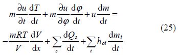
This equation has to be solved iteratively, and it is necessary to solve the following sub-models.

1)Gas properties model:

where A_j is found in JANAF thermodynamic tables(Chase et al., 1985). For a mixture of m species, the global internal energy is calculated using the fraction method:

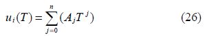
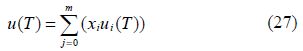
The same method is commonly used to calculate the specific stagnation enthalpy h.

2)Mass transfer model: The mass conservation equation is used to calculate the mass and the equivalence ratio evolution in the control volume which is the combustion chamber, as illustrated in Eqs.(28) and (29)(Guibert, 2005):

where int refers to intake air, exh refers to exhaust gas and inj refers to injected fuel.

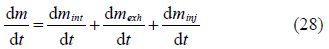
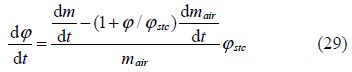
In Eq.(29)air refers to fresh air in the combustion chamber and stc refers to stoichiometric conditions.

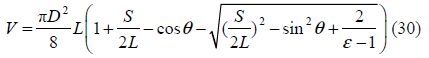
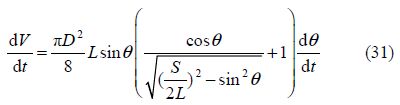
3)Kinematic model: The volume delimited by the piston, the cylinder wall and the cylinder head can be calculated as a function of the angular position of the crankshaft θ(Heywood, 1988):

Therefore, the volume variation can be calculated as a function of time:

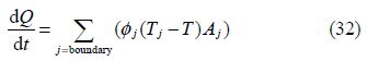
4)Heat transfer model:

Woschni(1967)has developed an empirical model to describe heat transfer through cylinder walls and piston. Eq.(32)gives the heat transfer through a boundary surface:

where ${{\phi }_{j}}$ is the exchange coefficient(Basbous et al., 2012).

5)Burn rate and combustion process model: The global combustion model can be simplified by the combination of two Wiebe laws(Stone, 1999). The first one describes the pre-mixed combustion and the second one describes the diffusion combustion.

Each Wiebe law allows the calculation of the burned fuel ratio as(Heywood, 1988):

where is the start of injection angle(SOI). The start of combustion(SOC)angle ${{\theta }_{SOC}}$ is the difference between ${{\theta }_{SOI}}$ and the AID(auto ignition delay)angle ${{\theta }_{AID}}$. Several equations are proposed in the literature review for modeling the AID. In this present work, it has been chosen to use the following equation developed by Hardenberg and Hase(1979) and recommended by Heywood(1988). where ${{\theta }_{AID}}$ is expressed in crank-degrees, v_p is the piston mean velocity(m/s), T is the temperature at top dead center(K), P is the pressure at top dead center(bar), E_a = 618 840/CN+25, where CN is the fuel cetane number.

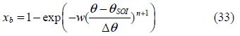
Parameters n and w of Eq.(33)are constants determined empirically. In this study, the values of n and w to 3 and 5 are set as found in literature review(Guibert, 2005), respectively. The combustion duration is calculated using the Taylor equation.

2.5.3 Experimental validation

In Fig. 12 the simulation results showed a real thermodynamic cycle(P-V diagram), the measured and esmtimated values of the cylinder pressure at W=1 440 r/min and T=1 120 N·m.

2.6 Gas emission 2.6.1 Description

The fuel combustion in a diesel engine, generates certain number of residues. These arise from complex chemical reactions of combustion and essentially depends on:

1)The fuel used;

2)The engine temperature;

3)The design of the combustion chamber;

4)The injection system;

5)Conditions of use.

Achieving a more complete combustion contributes to a minimum waste production. A perfect match between the maximum amount of fuel and air in the combustion chamber and an optimal mixing, limits the production of pollutants.

2.6.2 Model of thermodynamic cycle

A combustion process produces water(H₂O) and carbon dioxide(CO₂). It also produces in small amounts a series of undesirable compounds:

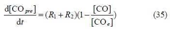
1)Carbone monoxide(CO).

The formation rate of CO in the premixed combustion stage can be expressed as(Heywood, 1988; Mansouri and Bakhshan, 2001):

where R_i(i=1, 2)is a rate of reaction at equilibrium, related to the temperature of combustion. The subscript e denotes the chemical equilibrium condition.

The formation rate of CO in the mixing controlled combustion stage can be expressed as(Roth et al., 1993):

where k_mix is a constant related to the portion of soot_o transformed to CO during the mixing controlled combustion stage.

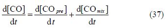
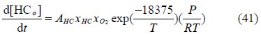
The emission rate of CO can be expressed as:

2)Unburned hydrocarbons(HC).

The HC emissions primarly come from two paths in diesel engine(Heywood, 1988; Ferguson and Kirkpatrick, 2001; Lakshminarayanan et al., 2002).

Overleaning:

where Q_ID is the quantity of fuel injected during ignition delay, related to the air-fuel ratio.

Undermixing:

where V_sac is the sac volume, x_sac is the fraction of fuel entering the cylinder from the sac. ρ_f is the fuel density.

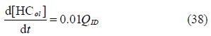
HC formation model:

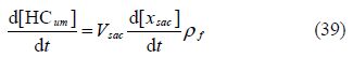
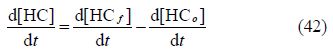
HC oxidation model:

where A_HC is an empirical constant, x_HC and are the mole fraction of HC and O₂.

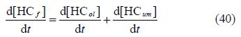
The net rate of unburned HC emissions:

3)Oxides of azote(NOx).

In the present model only the thermal mechanism(Zeldovich mechanism)(Heywood, 1988)is considered:

where R_i(i=3, 4)is a rate of reaction at equilibrium, related to the temperature of combustion. The subscript e denotes the chemical equilibrium condition.

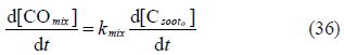
4)Soot particle.

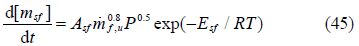
The net soot formation rate is calculated by using the model developed by Lipkea and DeJoode(1994):

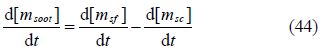
Soot formation:

Soot oxidation:

where A_sf, A_so are empirical constants to be adjusted in order to fit experimental emission data, n is a constant, $\dot{m}_{f,u}^{0.8}$ is the mass of unburned fuel vapor, P and T are the cylinder pressure and temperature, respectively, and E_sf, E_soare the activation energy for the soot formation and oxidation, is the oxygen partial pressure in the zone.

5)PM.

PM emissions are the sum of soot and SOF(Tan et al., 2007):

where the SOF is mainly the heavier fraction of HC emissions: where K_sh is a constant to be determined.

6)CO₂.

where 0.99 is the considered value for the combustion efficiency.

2.6.3 Experimental validation

Fig. 13 represent measured values of crankshaft rotaion speed(W) and the torque(T)that comm and the engine and shows the experimental and estimated values of the gas emissions.

3 Conclusion and perspective

A marine diesel engine model predicting pressure, temperature, efficiency, fuel rate, emissions, heat release at different point of the engine has been constructed. The engine is divided into subsystems: cooling, lubricating, injection, emission, air system and combustion. Each of them are discussed separately, then merged for building the dynamic model of the marine diesel engine. Some empirical and semi-empirical equations, are proposed in order to simplify the modeling, by which the accuracy and speed of the simulation are significantly improved. The simulation results showed that the simulation predictions are in agreement with the experiment.

In the future development of this research, the simulator can be used to investigate the impact on subsystems engine’s output of changing values of faults parameters for the most popular marine diesel engine faults like a faulty fuel injector, a leaky cylinder, a worn fuel pump, the broken piston rings, a dirty turbocharger, a dirty air filter, a dirty air cooler and many others. An application of this model such as diagnostic for the air system is achieved by Nohra et al.(2009). Thus, the simulator can be used, to study the diagnostics and prognostics of faults in all subsystems of the diesel engine.