


 , , , ,
2. South China Sea Marine Engineering Surveying Center, State Oceanic Administration, Guangzhou 510300, China;
3. China National Offshore Oil Corporation General Research Institute, Beijing 100027, China
1 Introduction
Local scour around offshore pipelines has significant effect on the stability of structure. Underst and ing the scouring processes and predicting the scour around pipelines are important in the design of offshore pipelines(Whitehouse, 1998). Because of the highly variable marine environment caused by waves, tidal and littoral currents, variability of sediments, etc., the scour around offshore pipelines is difficult to predict.
Over the last three decades, more and more numerical models for scour prediction have been developed. Based on the potential flow theory(Hansen et al., 1986; Mao, 1986), k-ε model(Leeuwenstein and Wind, 1984), morphological model(Li and Cheng, 2000), and smagorinsky subgrid scale(SGS)model(Liang et al., 2005)were put forward. Dey and Singh(2007)developed a semi-theoretical model for the computation of maximum clear-water scour depth that occurs below the underwater pipelines in uniform sediments under steady flows. Two-phase models considering the dynamics of particle and fluid phases as well as its interactions have been employed for sediment transport calculations in the framework of Navier-Stokes equations. In recent years, Zhao and Cheng(2008)solved the Reynolds-averaged Navier-Stokes equations and the transport equation for suspended sediment concentration by using a finite element method. The bed scour profile is determined through solving sediment mass conservation equation. The numerical model is validated against experimental data available in literature on scour below a single pipeline. Yang et al.(2008)established the similarity rules for modeling local scour under the submarine pipeline by means of dimensional analytical method, and then modeled the physical phenomenon of the local scour of the pipeline in a unidirectional flow flume. Zhang et al.(2009)analyzed the current field and the dimensionless shear stresses of the top and the bottom of the pipeline on the bed. The present numerical experiments(Zhao and Fernando, 2007; Zhao and Cheng, 2010)show that water depth has weak effect on the scour depth. However, it does affect the time scale of the scour. The shallower the water depth is, the less time it requires to reach the equilibrium state of scour. And so, it is intended to narrow the scope of study in this numerical simulation.
In order to take insight into the mechanism of pipeline erosions, it needs to analyze the underflow and the sediment motions around the pipelines. In the present study, the main work is to investigate the erosion of offshore pipeline in shallow water environments. Seabed erosion and the action of currents have a significant influence on the structural stabilities and erosion of the pipelines. An Eulerian two-phase model is employed to simulate the scour around pipelines. The aim is to evaluate the model’s efficacy using available benchmark data and , if successful, to use the model to educe important information on flow dynamics, which could not be conveniently obtained with available laboratory techniques, especially. Meanwhile, based on formulas of incipient velocity of sediments, approximate calculation on theoretical scour depths are put forward for seven stations in the South China Sea, which is available for engineering application information. According to the results of previous studies(Zhao and Fernando, 2007; Wei and Ye, 2008; Tan et al., 2010; Yang et al., 2013), they can be further applied to the actual process of engineering.
2 Numerical modelThe Eulerian multiphase flow model is capable of simulating multiple phase flow separation and interactions. Under the Eulerian multiphase flow framework, the flow is described as interacting continuum media with its volume fractions denoted by αt (t=w,s). The volume fraction is defined as the space ratio occupied by each phase. The laws of conservation of mass and momentum are satisfied by each phase, respectively. Coupling among phases is achieved through pressure and interphase exchange coefficients. A symmetric drag model is employed to describe the interaction between phases.
2.1 Governing equations
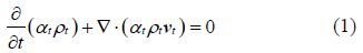
The continuity equation
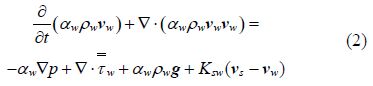
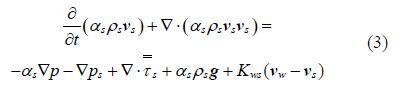
Momentum equations for water-water and water-sediment interactions
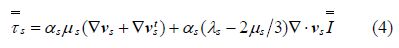
Stress tensor for the sediment phase is given by
Stress tensor for the water phase is given by
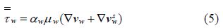
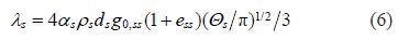
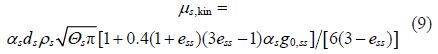
In Eq.(5),${{\mu }_{w}}$ is shear viscosity of water. The collisional and kinetic parts, and the optional frictional part, are added to give the sediments shear viscosity


The expression for the kinetic part is
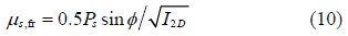
In dense flows at low shearing rate, where the volume fraction of the secondary phase, namely sediment phase, approaches its packing limit, the formation of the stress is mainly due to friction between particles. The frictional viscosity can be estimated by
The water-sediment exchange coefficient has the form

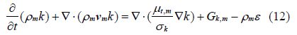
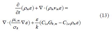
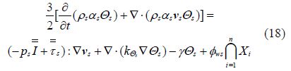
The k and $\varepsilon $ equations for the turbulence flow are as follows:


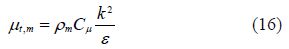
The turbulent viscosity ${{\mu }_{t,m}}$ is computed from
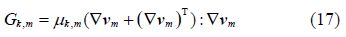
The production of turbulence kinetic energy ${{G}_{k,m}}$ is computed from
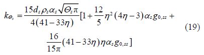
The granular temperature for the sediment phase is proportional to the kinetic energy of the r and om motion of particles. The transport equation derived from kinetic theory takes the form:
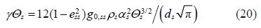
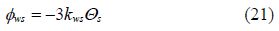
The transfer of the kinetic energy of r and om fluctuations in particle velocity from the sediment phase to the fluid phase is represented by ${{\phi }_{ws}}$:
For Eulerian multiphase model, the governing equations were solved using phase-coupled SIMPLE scheme for pressure-velocity decoupling. The first-order upwind discretization scheme was adopted for allusion of final results to volume fraction; the second-order upwind discretization scheme was adopted for the contraposed momentum, turbulent kinetic energy and dissipation rate.
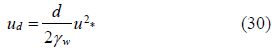
The dimensions of the computational domain are shown in Fig. 1. X is the streamwise direction, Y is the cross-stream direction and Dpipe(Diameter of the pipe)is the thickness of the s and layer. The water depth is dependent on Dpipe. According to Mao’s test(Mao, 1986), the influence of the pipe on the flow was taken into account and 4Dpipe was covered in the vertical direction, 5Dpipe and 15Dpipe from the center of the pipe for the inlet and outlet boundaries, respectively. In the beginning of the simulation, a sinusoidal profile with perturbation of amplitude 0.1Dpipe was adopted. The two-phase model configuration is described in Section 2.1-2.3 to simulate the real engineering conditions.

|
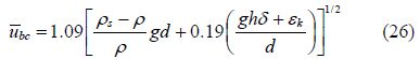
| Fig. 1 Computational domain and phase configuration |
A two-dimensional grid with 8 086 nodes and 7 869 elements was used. The grid consists of two zones, namely the water and the sediment zones. Non-uniform grid was adopted. During the simulations, the time step size was chosen based on the number of iterations per time step, which was considered 40 to obtain satisfactory results. The flow and turbulence equations were solved with a non-dimensional time-step dt = 0.001-0.1 s, and the volume fraction adopted dt = 0.01-0.1 s. Simulations showed that this time-step is small enough to ensure the solutions, and are independent on time-steps.
The steps for our simulation can be summarized as follows:
1)Generate the grid.
2)Use the mixture turbulence model in the FLUENT solver to calculate the fully developed velocity and turbulence for the fluid phase.
3)Use the Eulerian two-phase model in the FLUENT solver to calculate the solid-fluid interactions as well as the velocity of solid phase, using fully developed velocity from step 2)as the input.
The entire calculation process is controlled by an UDF(user defined function). The procedure was repeated until the equilibrium state of scour was reached.
The boundary conditions were defined as
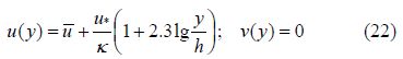
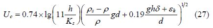
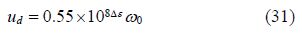
Fig. 2 shows the arrangement of position in the South China Sea in a real project. Flow characteristics for all of the stations listed in Table 1 were studied. The data obtained from in-site measurements were used for numerical simulations. The simulation results were applied in the engineering planning.

|
| Fig. 2 Position of key stations |
| Station | h/m | h'/m | u'/(m·s-1) | d50/mm | Dpipe/m |
| A2 | 100.4 | 1.29 | 0.650 | 0.247 | 0.838 8 |
| A3 | 173.1 | 1.445 | 0.400 | 0.146 | 0.845 2 |
| 25 | 77.3 | 13.5 | 0.500 | 0.060 | 0.838 8 |
| 28 | 54.5 | 6.6 | 0.450 | 0.039 | 0.858 8 |
| 29 | 54.5 | 6.6 | 0.450 | 0.356 | 0.858 8 |
| A1817 | 34 | 1.5 | 0.493 | 0.430 | 0.962 0 |
| A1607 | 28 | 1.9 | 0.540 | 0.009 | 0.962 0 |
The flow velocity will be changed when the pipeline is placed on the seabed. When the flow velocity is greater than erosion threshold, namely the incipient velocity, local scour will occur. Therefore, incipient velocity should be obtained firstly by comparing the simulation results against classical formulas.
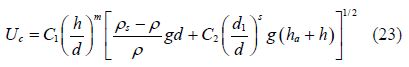
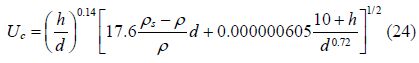
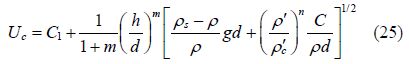
3.1 Zhang’s formula(Zhang, 2007)
By considering the characteristics of the instantaneous velocity, Dou(1999)proposed the formula
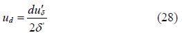
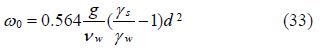
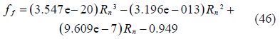
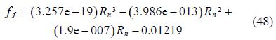
During the incipient motion of fine s and , particles are submerged within laminar boundary, whose velocity has a linear distribution, illustrated as Fig. 3.

|
| Fig. 3 Schematic diagram of fine s and and the velocity distribution |
According to Sha(1965), the relation between and $\Delta \varepsilon ={{\varepsilon }_{m}}-\varepsilon $ is

Combine the solution into Eqs.(31), (32) and (33), the critical drag resistance for fine s and can be derived as

Shields’ critical stress formula


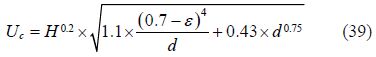
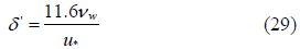
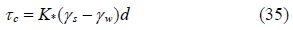
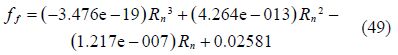
If the flow velocity near the pipeline is large enough to cause erosion, then the sediment will be gradually corroded as shown in Fig. 4.

|
| Fig. 4 Schematic diagram of the maximum scour depth(R=pipe radius, H=scour depth from the center of the pipe) |
The maximum scour depth is proposed by Chao and Hennessy(1972). This method provides an order-of-magnitude estimation of the possible scour hole depth. The subsurface current is assumed to flow perpendicular to the longitudinal axis of the pipeline. Based on the two-dimensional potential flow theory and the assumptions, the discharge through the scour hole is
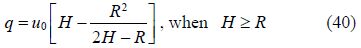
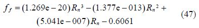
Once the flow velocity inside the scour hole is greater than the outside, erosion phenomenon appeared. As the expansion continues at erosion section, erosion will finally reach the quasi-equilibrium state. In the eroded trench, the boundary shear stress was calculated by the conditions assumed by Chao and Hennessy(1972). The friction coefficient ${{f}_{f}}$ can be estimated according to the Reynolds number defined by Lovera and Kennedy(1969)
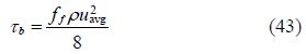

|
| Fig. 5 Prediction chart of friction coefficient in alluvial channel of flat ocean current |
According to different pipe diameters and particle sizes, the relation between ${{f}_{f}}$ and ${{R}_{n}}$ can be known by interpolation and fitting according to the friction coefficient predicted through the Table 2 and the Fig. 5. After solving the equations, the results are performed as follows:
| D50/mm | τc/(Lb/ft2) | D50/mm | τc/(Lb/ft2) |
| 0.05 | 0.016 1 | 0.50 | 0.021 5 |
| 0.08 | 0.016 2 | 0.75 | 0.026 6 |
| 0.10 | 0.016 4 | 1 | 0.031 6 |
| 0.13 | 0.016 6 | 2 | 0.051 3 |
| 0.25 | 0.017 2 | 4 | 0.089 0 |
1)Station A2:
2)Station A3:
3)Station 25:
4)Station 28:
5)Station 29:
6)Station A1817:
H and H-R can be solved by combining the above equations simultaneously. The A1607 station’s curve is beyond the scope of the graphics, therefore additional calculations are conducted, and the negative results are taken for scour depth to maintain numerical consistency.
3.7 Shields’ parameterShields’ parameter was used to determine the incipient motion of the sediment. After the Shields’ parameter $\varphi >{{\varphi }_{c}}$ bedload, then the transport would occur. Four depths have been considered in the article, namely the simulated water depth, actual water depth in fresh water, and the simulated water depth, actual water depth in sea water, respectively. Through estimation, the conclusions are drawn that all of actual Shields’ parameters are larger than the critical Shields’ parameters in the context of simulated water depth of fresh water, actual water depth of fresh water, simulated sea water depth of sea water, and actual water depth of sea water. Sediment erosion will occur.
4 Results and discussionThe scour calculations presented here are for the case with a cylinder of D = 0.1 m, the s and particle with d = 0.36 mm, Shields’ parameter θ = 0.048 according to experiment by Mao(1986). Experimental results(Fig. 6)were obtained by profiles measured, for the same conditions about clear-water scour case, simulated scour depth results match to experiment results. It provides important information for the improvement and optimization of the pipeline design. Although the decay of turbulence due to energy releasing process and the motion of particles tends to pile up s and behind the pile, the current situation is difficult to control the mound owing to particles will be accumulated at the rear of the tank. In view of these characteristics, to some scour development along with pipelines, the time is unsuitable between the predictions and the experiments.

|
| Fig. 6 Bed profiles during pipeline scour |
The current and wave-induced flow scouring around the submarine pipelines greatly endangers engineering safety. Meanwhile, the pipeline will also cause local hydrodynamic environment changes. The simulation results showed that for small initial depth of submarine pipeline, considering only unidirectional currents caused by local scour, is usually divided into four phases, suspended pipeline, gap scour, wakefield scour and equilibrium scour. The location of maximum scour depth is at the downstream side of the pipe under the condition of limit equilibrium scour. Along with the narrowing of the initial gap between the pipeline and s and bed, equilibrium scour depth increases. Around the pipeline, strong wakes and vortexes usually occur, which cause local non-equilibrium sediment transport, resulting in even stronger scour around the pipeline. For the sea area with relatively deep water, tidal flow is thought to be the main factor that induces local scour.
The single-phase velocity field of the flow was calculated with an updated bed form. Based on the typical flow(Fig. 7), the final results can be obtained gradually. Through calculation and dynamic adjustment of the distribution factor for sediment concentrations, more accurate suspended-load flow change can be obtained. Only those that are really taken into account can be estimate, so the scour depth in the simulation is constrained by the attention span. Fig. 8 presents the variation of bed profiles(stations from A2 to A1607)in the two-phase flow simulation. As mentioned, the volume fraction of sediment contour ≈ 0.5 was chosen as the bed profiles by using Tecplot software for post processing.

|
| Fig. 7 Typical flow field and sediment concentration |

|
| Fig. 8 Bed profiles during the development of scouring |
To optimize the problem of scour, the multiple “2 stages” optimization method was put forward. The multiphase flow problem was solved by trying to occupy a space water condition between seabed and pipeline. However, it must be ensured that the flow is fully developed through the initial calculation of the flow field to update the bed and so on. When the maximum change of scour depth along the sediment-water interface becomes smaller and smaller, more optimized results will be obtained. The flow velocity in front of the pipeline decreases due to the existence of the pipeline, which results in higher velocity around the pipeline, especially at the bottom of seabed. If the flow velocity of rising tide is bigger than the incipient velocity of sediment, the sediment particles will eject rapidly away from the bed surface in the form of the bed load and part of the suspended load. Energy dissipates during this process in terms of the distance from the pipeline. More and more sediment particles are deposited to form a mound due to the concentration of the bed in motion. The point to note is that calculations must satisfy the laws of incipient motion for sediment. The results showed familiarity with the theories about the development mechanism of scour within a reasonable control range. In the next place, vertical section increases gradually with the increase of scour depth, local velocity deceases rapidly, turbulence is reduced and alleviated, and streamlines constantly update with changes in terrain and drive the movement of particles until the last local steady state. The existence of the downstream dune can’t be seen attributed to sediment itself or the calculation is excessively sketchy in the balance process. Ultimately, the equilibrium profile is reached and the scour depth to an approximate dynamic equilibrium situation that is interesting will be used as a reference value.
The present study provides the approximate state of sediment erosion including the sediment(29 and A1817 stations), fine sediment(A2 and A3 stations), extra fine sediment(25 and 28 stations), silt(A1607 station). However, the forecast is done before construction and the verification of reliability, but the so experiment is not done for validation although the actual conditions in worksite should be satisfied. For comparison, the early scour results on seven different stations are listed, which is mainly to explore the influence of sediment size on seabed pipeline. Different initial mean velocity with the current case plays a certain reference arriving role to scour evolution around pipelines. In these stations, the maximum mean velocity of vertical sections belongs to A2 station, with the minimum diameter of the pipe, the scour pit pattern and maximum scour depth are the characters which can be found easily on the fine sediment.
4.2 Scour depthFig. 9 presents a plot of scour depth(stations from A2 to A1607)as a function of time. A faster scouring rate during the period between 10 and 100 minutes indicates that the bottom layer depth determines the initial scour rate. The solid line shown indicates that the scour depth no longer changes after 50 minutes and the scour pit is in balance. The effects of incipient velocity, pipe diameter and sediment particle size are considered simultaneously in analyzing the incipient of sediment around the pipeline. The scour depth of 28 and A1607 stations shows a general reasonableness for sediment particle size distribution. When sediment particle size is small to a certain extent, the bed surface sediment gradually becomes difficult to start. This can be reflected in the s and (25 stations). When the sediment particle size is large to a certain extent, the situation is not different, which results in the size of the relevant response for scour depth. Scour depth increases with time and then tends to limit the final equilibrium state.

|
| Fig. 9 The time evolution of scour depth in simulations |
As mentioned above, six theoretical formulas(Table 3)were chosen in the tests. Those formulas were chosen to achieve a relatively broad scour depth range. The calculations were also carried out for the same pipe diameter. The results were validated by numerical results, indicating that the theoretical results can't meet the actual requirements under the action of currents. As seen in Table 8, when the scour depth becomes a certain value(greater than 1 m), this case is considered as “Deposit”. Compared to all cases, deposit and scour around the pipeline is complex, in which vortex results in intense erosion. However, it could not be greater than 1 m according to the experimental results(Mao, 1986) and the actual conditions in worksite in the South China Sea. The present model predicts that this is a little smaller than the theoretical results, respectively. The stations for 25, 28 and 29 are predicted to be too low when compared with others indicated. This may be a result of the fact that the theoretical results could be calculated to provide slightly too much deposition due to the limit of the conditions in theoretical formula.
| m | |||||||
| Method | A2 | A3 | 25 | 28 | 29 | A1817 | A1607 |
| Zhang | −0.93 | −0.16 | Deposit | Deposit | 0.06 | −0.33 | 0.72 |
| Tang | 0.30 | 0.74 | Deposit | Deposit | Deposit | 0.62 | 0.72 |
| Dou | −1.09 | −0.16 | Deposit | Deposit | 0.069 | −0.53 | 0.87 |
| Wang and Bai | −0.47 | 0 | Deposit | Deposit | Deposit | 0.18 | 0.87 |
| Sha | −0.35 | 0 | Deposit | Deposit | Deposit | 0.07 | 0.85 |
| Herbich | −0.38 | −0.89 | −0.68 | −1.01 | −1.13 | −0.32 | −0.38 |
| Present model | −0.53 | −0.35 | −0.35 | −0.35 | −0.30 | −0.40 | −0.49 |
The main purpose of this paper is to obtain resonable results from theoretical formula calculations and numerical simulation for pipeline scour. Considering the different sediment situations of seven stations, it can be found that the calculated results are significantly different. But in general, the scour depth around the pipeline is not very deep, and the maximum scour depth should be less than 1 m, which means that the scour depth will not exceed the pipe diameter. In the simulations, erosion processes showed the dependence on the calculated curve model selection, but the ultimate limit equilibrium scour depth was the same. It was far beyond any reasonable doubt that the calculated results agreed well with the obtained monitoring data during the construction of a foundation for pipeline in the South China Sea, which showed the reliability of mathematical models for scour prediction below offshore pipelines. The calculation results demonstrated that the numerical method presented in this article can meet the engineering application dem and . According to the test, the influence of incipient velocity, pipe diameter and sediment particle size on scour depth should be considered in combination with the theoretical analysis and numerical method, especially on such aspects as a huge project that the experiment can not be performed.
AcknowledgementWe wish to thank Prof. Bai YC for stimulating discussions and reviewers for their helpful comments that led to considerable improvements to the paper.
| Chao JL, Hennessy PV (1972). Local scour under ocean outfall pipelines. Journal of the Water Pollution Control Federation, 44(7), 1443-1447. |
| Dey S, Singh NP (2007). Clear-water scour depth below underwater pipelines. Journal of Hydro-environment Research, 1(2), 157-162. DOI:10.1016/j.jher.2007.07.001 |
| Dou GR (1999). Incipient motion of coarse and fine sediment. Journal of Sediment Research, (6), 1-9. (in Chinese) DOI: 10.3321/j.issn:0468-155X.1999.06.001 |
| Hansen EA, Fredsoe J, Mao Y (1986). Two-dimensional scour below pipelines. Proc. 5th Int. Symp. on Offshore Mech. and Arctic Eng., New York, 3, 670-678. |
| Herbich JB (1981). Offshore pipeline design elements. Marcel Dekker, Inc., New York, 41-69. |
| Jiang CB, Bai YC, Jiang NS, Hu SX (2001). Incipient motion of cohesive silt in the Haihe River estuary. Journal of Hydraulic Engineering, 32(6), 51-56. (in Chinese) |
| Leeuwenstein W, Wind HG (1984). The computation of bed shear in a numerical model. Proceedings of 19th Conference on Coastal Engineering, Houston, USA, 2, 1685-1702. DOI: http://dx.doi.org/10.9753/icce.v19 |
| Li FJ, Cheng L (2000). Numerical simulation of pipeline local scour with lee-wake effects. International Journal of Offshore and Polar Engineering, 10(3), 195-199. |
| Liang DF, Cheng L, Li FJ (2005). Numerical modeling of flow and scour below a pipeline in currents: Part II. Scour simulation. Coastal Engineering, 52(1), 43-62. DOI:10.1016/j.coastaleng.2004.09.001 |
| Lovera F, Kennedy JF (1969). Friction-factors for flat-bed flows in sand channels. Journal of the Hydraulics Division, 95(4), 1227-1234. |
| Mao Y (1986). The interaction between a pipeline and an erodible bed. PhD thesis, Institute of Hydrodynamics and Hydraulic Engineering, Technical University of Denmark, Lyngby, Denmark. |
| Sha YQ (1965). Sediment mechanical dynamics. China Industry Press, Beijing, 167-168. (in Chinese) |
| Streeter VL (1963). Fluid mechanics. McGraw-Hill, New York, 33-75. |
| Tan GM, Jiang L, Shu CW, Lv P, Wang J (2010). Experimental study of scour rate in consolidated cohesive sediment. Journal of Hydrodynamics, Ser. B, 22(1), 51-57. DOI: 10.1016/S1001-6058(09)60027-5 |
| Tang CB (1963). Incipient motion of sediment. Journal of Hydraulic Engineering, (2), 1-12. (in Chinese) |
| Wang SY, Shen HW (1985). Incipient sediment motion and riprap design. Journal of Hydraulic Engineering, 111 (3), 520-538. |
| Wei YJ, Ye YC (2008). 3D numerical modeling of flow and scour around short cylinder. Chinese Journal of Hydrodynamics, 23(6), 655-661. (in Chinese) |
| Whitehouse R (1998). Scour at marine structures: A manual for practical applications. Thomas Telford Press, London, 45-58. |
| Yang B, Gao FP, Wu YX (2008). Experimental study on local scour of sandy seabed under submarine pipeline in unidirectional currents. Engineering Mechanics, 25(3), 206-210. |
| Yang B, Tao Y, Ma JL, Cui JS (2013). The experimental study on local scour around a circular pipe undergoing vortex-induced vibration in steady flow. Journal of Marine Science and Technology, 21(3), 250-257. DOI: 10.6119/JMST-012-0412-2 |
| Zhang CL, Yu GL, Xie JB (2009). The characteristics of the shear stress and flow field around a pipeline on fixed-bed with different gap-ratios in unidirectional flows. Marine Sciences, 33(3), 27-30. (in Chinese) |
| Zhang RJ, Xie JH, Chen WB (2007). River dynamics. Wuhan University Press, Wuhan, 32-37. (in Chinese) |
| Zhao M, Cheng L (2008). Numerical modeling of local scour below a piggyback pipeline in currents. Journal of Hydraulic Engineering, 134(10), 1452-1463. DOI:http://dx.doi.org/10.1061/(ASCE)0733-9429(2008)134:10(1452) |
| Zhao M, Cheng L (2010). Numerical investigation of local scour below a vibrating pipeline under steady currents. Coastal Engineering, 57(4), 397-406. DOI: 10.1016/j.coastaleng.2009.11.008 |
| Zhao ZH, Fernando HJS (2007). Numerical simulation of scour around pipelines using an Euler-Euler coupled two-phase model. Environmental Fluid Mechanics, 7(2), 121-142. DOI: 10.1007/s10652-007-9017-8 |