


 , ,
, ,
2. Department of Mechanical Engineering, Babol University of Technology, P.O. Box 484 Babol, Iran;
3. Department of Mechanical and Aerospace Engineering, Politecnico di Torino, 24-10129 Turin, Italy
1 Introduction
Viscoelasticity is the property of materials that exhibit both viscous and elastic characteristics when undergoing deformation. Viscous materials, like honey and s and , resistshear flow and strainlinearly with time when astressis applied. Elastic materials strain when stretched and quickly return to their original state once the stress is removed. Viscoelastic materials have elements of both of these properties.
The dynamic response of beams on viscoelastic foundations is an interesting problem in several fields of engineering. And several people have studied this problem. Since a minority of scientific problems has precise analytical solutions and most of the techniques like perturbation methods are not practical for strongly nonlinear equations. In recent years, much attention has been devoted to the newly developed manners to gain an approximate solution of nonlinear equations. This consists of: energy balance method(Sfahani et al., 2011; Momeni et al., 2011; Jamshidi and Ganji, 2010), homotopy analysis method(Das and Gupta, 2011; Pirbodaghi et al., 2009; Tari et al., 2007b; Domairy and Fazeli, 2009), He's amplitude frequency formulation method(HAFF)(He, 2008; Ren et al., 2009), parameter-expansion method(He, 2000; Kimiaeifar et al., 2010, Ganji et al., 2009b), EXP-function method(He and Wu, 2006; Chang, 2011, Alipour et al., 2011; Davodi et al., 2010; Ganji et al., 2009c; 2009d; Ganji and Abdollahzade, 2008), differential transformation method(DTM)(Ganji et al., 2010; Azimi et al., 2012; Joneidi et al., 2009), homotopy perturbation method(Ganji, 2006; He, 1999a; Fereidoon et al., 2010), adomian decomposition method and variational iteration method(He, 1998; 1999b; Tari et al., 2007a; Rafei et al., 2007). But the afore-mentioned methods do not have this ability to gain the solution of the presented problem in high precision. Therefore, these complicated nonlinear equations such as the presented problems in this paper should be solved by utilizing other approaches like AGM. AGM is a new approach for solving complicated nonlinear differential equations in various fields of study especially in mechanical and civil engineering(Clough and Penzien, 1975; Chopra, 1995; Ganji et al., 2009a).
AGM is a very suitable computational process and is usable for solving various nonlinear differential equations. Moreover, in AGM by solving a set of algebraic equations, complicated nonlinear equations can easily be solved and without any mathematical operations such as integration, the solution of the problem can be obtained very simply and easily. It is worthwhile to note that in AGM considering three or four sentences of the series of polynomials which are considered as the answer of differential equations is sufficient to obtain reliable solutions, and always by increasing the number of sentences the solution gets closer to the exact solution while in other methods the error might increase or decrease. For example, in this problem by adding a sentence to the series of polynomials the solutions get much more accurate. It is notable that this solution procedure, AGM, can help students with intermediate mathematical knowledge to solve a broad range of complicated nonlinear differential equations(Akbari et al., 2014a; 2014b; Ganji et al., 2014).
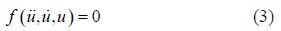
2 The analytical methodIn general, vibrational equations and their initial conditions are defined for different systems as follows:


In AGM, a total answer with constant coefficients is required in order to solve differential equations in various fields of study such as vibrations, structures, fluids and heat transfer. In vibrational systems with respect to the kind of vibration, it is necessary to choose the mentioned answer in AGM. To clarify here, we divide vibrational systems into two general forms.
2.1.1 Vibrational systems without any external forceDifferential equations governing on this kind of vibrational systems are introduced in the following form:

According to trigonometric relationships, Eq.(4)is rewritten as follows:
Sometimes for increasing the precision of the considered answer of Eq.(3), another term in the form of cosine by inspiration of Fourier cosine series expansioncan be added as follows:

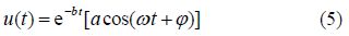
In the above equation, the term $({{\rm{e}}^{ - b\,t}})$ is omitted to facilitate the computational operations in AGM if the system is considered without any damping components.
Generally speaking in AGM, Eq.(5)or Eq.(6)is assumed as the answer of the vibrational differential Eq.(3)that its constant coefficients which are $a\,,\,\,b\,,\,\,d\,\,,\omega $ (angular frequency) and $\varphi$ (initial vibrational phase)can easily be obtained by applying the given initial conditions in Eq.(2). Also, the above procedure will completely be explained through the presented example in the foregoing part of the paper.
It is noteworthy that if there is no damping component in the vibrational system, the constant coefficient of b in Eq.(5) and Eq.(6)will automatically be computed zero in AGM solution procedure. On the contrary, the parameter b in Eq.(5) and Eq.(6)for the other kind of vibrational system with damping component is obtained as a nonzero parameter in AGM.
2.1.2 Vibrational systems with external forceIn this step, it is assumed that the external forces exerting on the vibrational systems are defined as:
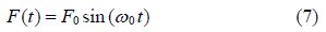
As a result, the differential equation governing on the vibrational system is expressed like Eq.(1)as follows:

The answer of the above equation is introduced as the sum of the particular solution(up) and the harmonic solution(uh)as follows:
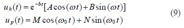

In order to increase the precision of the achieved equation, another term in the form of cosine by inspiration of Fourier cosine series expansionis added as follows:
Finally, the exact solution of the all vibrational differential equations can be obtained in accordance with the following equation:
To deeply underst and the above procedure, reading the following lines is recommended:
Since the constant coefficient(b)in vibrational systems without damping components is always obtained zero, we can add the term(bt)instead of $({{\rm{e}}^{ - bt}})$ in Eq.(12)to decrease computational operations in the following form:

Based on the above explanations, by applying initial conditions on a system without damping component, the value of parameter(b)is always zero for Eq.(12) and Eq.(13). Therefore, the role of parameter(b)in the both of Eq.(12) and Eq.(13)where each of them can be considered as the answer of the vibrational problems is individually considered as a catalyst for increasing the precision of the assumed answer. However, according to Eq.(15) and Eq.(19)after applying initial conditions on the vibrational system in both states(with external force and without external force)by AGM, the value of parameter(b)is computed zero because the mentioned system has a free vibration without any damping component.
The investigation showed that in order to decrease computational operations for systems without damping component that(b)in the term $({{\rm{e}}^{ - bt}})$ is zero so $({{\rm{e}}^{ - bt}})$ can be omitted from Eq.(11). Consequently, Eq.(11)which has been considered as the answer of the systems without any damping component can be rewritten as follows:

The constant coefficients of Eq.(11)or Eq.(12)which are $\left\{ {a,\,\,b,\,\,\omega ,\,\,\varphi ,\,\,c,d,\,\,\phi } \right\}$ will easily be computed in AGM by applying the initial conditions of Eq.(2).
2.2 Application of initial conditions to compute constant coefficients and angular frequency by AGMIn AGM, the application of initial conditions of Eq.(2)is done in the two following forms.
2.2.1 Applying the initial conditions on the answer of differential equationIn regard to the kind of vibrational system(with external force and without external force), a function is chosen as the answer of the differentialequation from Eq.(5)or Eq.(6)for the systems without external forces and from Eq.(11)or Eq.(12)for the defined systems with external forces and then the initial conditions are applied on the selected function as follows:
It is notable that IC is the abbreviation of introduced initial conditions of Eq.(2).
2.2.2 Appling the initial conditions on the main differential equation and its derivativesThe best time to substitue the mentioned answer into the main differential equation instead of its dependent variable(u)is after choosing a function as the answer of differential equation according to the kind of vibrational system.
Assume the general equation of the vibration such as Eq.(1)with time-independent parameter(t) and dependent function(u)as:

Therefore, on the basis of the kind of vibrational system, a function as the answer of the differential equation such as Eq.(5)or Eq.(6) and Eq.(11)or Eq.(12)are considered as follows:

Eventually, the application of initial conditions on Eq.(18) and its derivatives is expressed as:
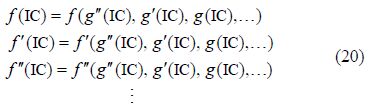
Eq.(20)means that the initial conditions(or boundary conditions)of the differential equation can be developed. In other words, to calculate the constants of the solution function(Eq.(11)or Eq.(12))a set of algebraic equations need to be solved first(with an equal number of algebraic equations and number of unknowns). After substituting Eq.(18)in the differential equation and successive differentiation(if needed), make the number of algebraic equations equal to the number of unknowns of solution function. The coefficients of solution function()can be easily achieved by solving the set of algebraic equations.
In AGM, after applying the initial conditions of Eq.(17), Eq.(18) and also on its derivatives from Eq.(19)according to the order of differential equation and utilizing the own two given initial conditions of Eq.(2), a set of algebraic equations of n equations with n unknowns is created. Therefore, the constant coefficients(a, b, c, d, angular frequency "$\omega$" and initial phase)are easily achieved which this procedure will thoroughly be explained in the form of an example in the foregoing part of this paper.
It is noteworthy that in Eq.(19), derivatives of with higher orders until the number of yielded equations is equal to the number of the mentioned constant coefficients of the assumed answer can be used.
3 Application of AGMThe rigid beam shown in Fig. 1 with a pin support in the middle on the viscoelastic foundation is modeled with spring stiffness of(k) and damping coefficient of(c)per unit length. The vibrational equation and angular frequency for great anglesis obtained as showed in Fig. 1. Fig. 2 shows the forces acting on the vibrating rigid beam shown in Fig. 1.

|
| Fig. 1 The schematic of the rigid beam with a pin support on the viscoelastic foundation |

|
| Fig. 2 The displacement diagram of the mentioned system |
The point O which is the pin support as follows:

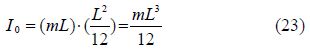
The mass moment of inertia of the mass per unit length of the rigid beam is as follows:
The initial conditions for Fig. 1 according to Eq.(26)are expressed in the forms of:

Before starting the solution procedure, it is necessary to mention that in order to solve nonlinear differential equation by AGM there is no need to use Taylor series expansion for the term $(\sin \theta \,)$ whereas in the other methods such as EBM, VIM and PMM, which convert the trigonometric terms into their Taylor series expansions(Ganji, 2006; Ganji et al., 2009b). As a result, the obtained solution by AGM is more accurate and precise in comparison with the afore-mentioned methods. For solution of Eq.(26)in AGM, a polynomial and trigonometric function is as follows:
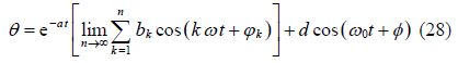
Term($d\cos \left( {{\omega }_{0}}t+\phi \right)$)in Eq.(28)is related to external forces applied to the system that does not exist in this problem. For answer of differential equation with acceptable accuracy a term of answer function(n=1)can be chosen as follows:
The constant coefficients of Eq.(29), ω, φ, a and b can easily be obtained by applying the initial conditions.
3.2 Applying initial conditions in AGMIt is noteworthy that in the proposed method, initial or boundary conditions are applied in 2 ways as follows:
1)In general, the initial conditions are applied on Eq.(28)in the form of:
For simplicity, IC is considered as the abbreviation of the initial conditions. As a result, applying the initial conditions on Eq.(30)is done as:


2)The application of initial or boundary conditions on the main differential equation which in this case is Eq.(26) and also on its derivatives is done in the following general form:

Therefore, after substituting Eq.(29), which has been considered as the answer of the main differential equation, into Eq.(26), the initial conditions are applied on the obtained equation and also on its derivatives on the basis of Eq.(32)as follows:
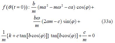
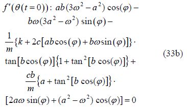
Solving a set of algebraic equations that consist of: four equations, four unknowns(from Eq.(31a), Eq.(31b), Eq.(33a), and Eq.(33b)) and constant $a\,,\,\,b\,,\,\,\varphi \,\,$ coefficients and $\omega$ (from Eq.(29))the following can be yielded:
To simplify, the following new variable are introduced as:
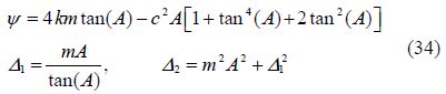
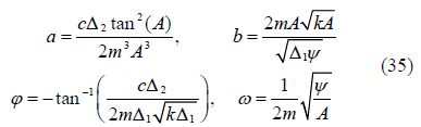
After substituting the obtained values from Eq.(35)into Eq.(29), the solution of nonlinear differential Eq.(26)by AGM will be obtained as follows:
By selecting the following physical quantities for Fig. 1:


Then, the charts of the obtained solution function, its derivative and its phase plane are drawn in Figs. 3-5.

|
| Fig. 3 The obtained solution by AGM |

|
| Fig. 4 The derivative of the obtained solution by AGM |

|
| Fig. 5 The resulted phase plane by AGM |
With regard to the given physical values from Eq.(37) and the determined domain which is defined in terms of second(s), the solution of the differential equation is expressed numerically(Runk45)in Table 1.
| t/s | Error/% | t/s | Error/% | ||||||
| 0 | 0.2 | 0.2 | 0.00 | 0.0 | 48 | −0.050 518 11 | −0.050 635 71 | 0.23 | −0.013 339 7 |
| 16 | 0.090 485 15 | 0.090 753 42 | 0.29 | −0.046 517 2 | 64 | −0.038 655 24 | −0.038 728 01 | 0.18 | 0.006 100 332 |
| 32 | −0.011 689 17 | −0.011 547 80 | 1.20 | −0.039 488 1 | 80 | −0.011 016 078 | −0.011 240 90 | 2.04 | 0.011 298 127 |
Due to the obtained solution from Eq.(36)by AGM and the obtained numerical solution, which its results have been presented in Table 1, the following comparisons are provided at Figs. 6-8.

|
| Fig. 6 A comparison between the achieved solutions by AGM and numerical method |

|
| Fig. 7 A comparison between the derivative of the achieved solutions by AGM and numerical method |

|
| Fig. 8 Comparing the resulted phase planes by AGM and numerical method |
The following Figs. 9 and 10 are the difference between the results on the basis of the yielded solution from Eq.(36)by AGM and the results of Table 1 by numerical method.

|
| Fig. 9 Comparing the absolute differences between displace-ment functions which are predicted by AGM and numeric method |

|
| Fig. 10 Comparing the absolute differences between velocity functions which are predicted by AGM and Numeric method |
With regard to theFigs. 9 and 10, it is revealed that the errors increase rapidly until t = 50 s and after that decrease steadily.
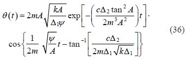
3.6 Results and discussion 3.6.1 The angular frequency(ω)The angular frequency (ω) from Eq.(35)in terms of initial amplitude of vibration is seen at Fig. 11. It is clear that the more amount of amplitude of vibration in the initial condition(IC), the more increasing of the angular frequency.

|
| Fig. 11 The chart of angular frequency in terms of initial vibrational amplitude |
The damping factor in the vibrational solution of $b\left\{ {{\text{e}}^{-at}}\cos (\omega t+\varphi ) \right\}$ is ${{\text{e}}^{-at}}$ since in the vibrational differential equation the term is the main factor for damping, ($\xi $) can be obtained as follows:
The damping ratio ($\xi $) in terms of initial amplitude of vibration from Eq.(39)is depicted in Fig. 12.

|
| Fig. 12 The variation of damping ratio in terms of the initial amplitude of vibration(A) |
With regard to the Fig. 12, it is revealed that by increasing the amount of initial amplitude of vibration (A), the value of damping ratio will be increased. Therefore in this step, it is logical to indicate that inasmuch as the formula of damping coefficient is obtained by $c=2m\,\omega \,\xi$ , there is a direct relationship between initial amplitude of vibration and damping coefficient.
3.6.3 Energy lost per cycleEnergy dissipated per cycle by the damping force(Fd)can be shown with graphical display. Terms of damping force in the differential Eq.(26)is obtained as follows.
After insertion of the derivative of Eq.(36)into Eq.(40)the following result is obtained:


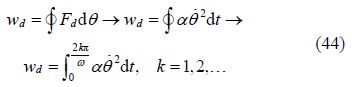
For each cycle of vibration at times($t=\frac{2k\text{ }\!\!\pi\!\!\text{ }}{\omega }\,,\,\,\,k=1\,,\,\,2\,,\,...\$)with the merger of the two equations Eqs.(41) and (42), the trigonometric relations damping force can be obtained as follows:
As well as the energy lost per cycle of vibration, the equation is as follows:
The comparison of the energy loss for three cycles is depicted in Figs. 13-16. They show that the energy lost per cycle is determined by the area enclosed by the ellipse.

|
| Fig. 13 Energy dissipated in the first cycle(k=1) |

|
| Fig. 14 Energy dissipated in the second cycle(k=2) |

|
| Fig. 15 Energy dissipated in the third cycle(k=3) |

|
| Fig. 16 Energy dissipated in the third cycle(k=1, 2, 3) |
In this paper, a rigid beam with pin support on the viscoelastic foundation has been modeled. The complicated nonlinear vibrational differential equations governing it have been introduced and analyzed by AGM and the results have been compared with numerical method(Runk45). This problem was solved analytically and the solution is obtained for different values of frequencies and amplitudes. This showed that by increasing the amplitude of vibration in initial condition the angular frequency and the value of damping ratio increases. The dissipated energy in different cycles was also investigated. The above process has been done in order to show that AGM can be used for solving a broad range of differential equations in different fields of study particularly in vibrations. Consequently, it is concluded that AGM is a reliable and precise approach for solving differential equations. Moreover, a summary of the AGM excellence and benefits is explained. By solving a set of algebraic equations with constant coefficients, it is possible to obtain the solution of nonlinear differential equation along with the related angular frequency simultaneously easily. Applying this procedure is possible even for students with intermediate mathematical knowledge. On the other h and , it is better to say that AGM is able to solve linear and nonlinear differential equations directly in most of the situations. This means that the final solution can be obtained without any dimensionless procedure. Therefore, AGM can be considered as a significant progress in nonlinear sciences. The shortage of boundary condition(s)in this methodfor solving differential equation(s)is completely terminated. AGM is operational for nonlinear differential equations especially for the vibrations of civil engineering and mechanical engineering.
AcknowledgementThe authors are grateful to the Ancient Persian mathematician, astronomer and geographer Muhammadibn Musa Kharazmi who was the one that his Compendious Book on Calculation by Completion and Balancing presented the first systematic solution of linear and quadratic equations. Furthermore, he has been considered as the original inventor of algebra and is the one who Europeans derive the term ALGEBRA from his book and also the expression ALGORITHM has been taken from his name(the Latin form of his name). Consequently, we dedicate this way of solving linear and nonlinear differential equations to this scientist.
| Akbari MR, Ganji DD, Ahmadi AR, Hashemikachapi SH (2014a). Analyzing the nonlinear vibrational wave differential equation for the simplified model of tower cranes by (AGM). Frontiers of Mechanical Engineering, 9(1), 58-70. DOI: 10.1007/s11465-014-0289-7 |
| Akbari MR, Ganji DD, Majidian A, Ahmadi AR (2014b). Solving nonlinear differential equations of Vanderpol, Rayleigh and Duffing by AGM. Frontiers of Mechanical Engineering, 9(2), 177-190. DOI: 10.1007/s11465-014-0288-8 |
| Alipour MM, Domairry G, Davodi AG (2011). An application of exp-function method to approximate general and explicit solutions for nonlinear Schrödinger equations. Numerical Methods for Partial Differential Equations, 27(5), 1016-1025. DOI: 10.1002/num.20566 |
| Azimi MR, Ganji DD, Abbasi F (2012). Study on MHD viscous flow over a stretching sheet using DTM-Pade’ Technique. Modern Mechanical Engineering, 2, 126-129. DOI: 10.4236/mme.2012.24016 |
| Chang JR (2011). The exp-function method and generalized solitary solutions. Computers & Mathematics with Applications, 61(8), 2081-2084.. DOI: 10.1016/j.camwa.2010.08.078 |
| Chopra AK (1995). Dynamic of structural: Theory and application to earthquake engineering. Prentice-Hall Inc., Englewood Cliffs, USA, 07632. |
| Clough RW, Penzien J (1975). Structural dynamic. McGraw-Hill, New York, 430-438. |
| Das S, Gupta P (2011). Application of homotopy analysis method and homotopy perturbation method to fractional vibration equation. International Journal of Computer Mathematics, 88(2), 430-441. DOI: 10.1080/00207160903474214 |
| Davodi AG, Ganji DD, Davodi AG, Asgari A (2010). Finding general and explicit solutions (2+1) dimensional Broer-Kaup-Kupershmidt system nonlinear equation by exp-function method. Applied Mathematics and Computation, 217(4), 1415-1420. DOI: 10.1016/j.amc.2009.05.069 |
| Domairy G, Fazeli M (2009). Homotopy analysis method to determine the fin efficiency of convective straight fins with temperature-dependent thermal conductivity. Communications in Nonlinear Science and Numerical Simulation, 14(2), 489-499. DOI: 10.1016/j.cnsns.2007.09.007 |
| Fereidoon A, Rostamiyan Y, Akbarzade M, Ganji DD (2010). Application of He’s homotopy perturbation method to nonlinear shock damper dynamics. Archive of Applied Mechanics, 80(6), 641-649. DOI: 10.1007/s00419-009-0334-x |
| Ganji DD (2006). The application of He’s homotopy perturbation method to nonlinear equations arising in heat transfer. Physics Letters A, 355(4-5), 337-341. DOI: 10.1016/j.physleta.2006.02.056 |
| Ganji DD, Abdollahzade M (2008). Exact travelling solutions for the Lax’s seventh-order KdV equation by sech method and rational exp-function method. Applied Mathematics and Computation, 206(1), 438-444. DOI: 10.1016/j.amc.2008.09.033 |
| Ganji DD, Akbari MR, Goltabar AR (2014). Dynamic vibration analysis for non-linear partial differential equation of the beam-columns with shear deformation and rotary inertia by AGM. Development and Applications of Oceanic Engineering (DAOE), 3, 22-31. |
| Ganji DD, Malidarreh NR, Akbarzade M (2009a). Comparison of energy balance period with exact period for arising nonlinear oscillator equations: He’s energy balance period for nonlinear oscillators with and without discontinuities. Acta Applicandae Mathematicae, 108(2), 353-362. DOI: 10.1007/s10440-008-9315-2 |
| Ganji SS, Ganji DD, Babazadeh H, Sadoughi N (2010). Application of amplitude-frequency formulation to nonlinear oscillation system of the motion of a rigid rod rocking back. Mathematical Methods in the Applied Sciences, 33(2), 157-166. DOI: 10.1002/mma.1159 |
| Ganji SS, Sfahani MG, ModaresTonekaboni SM, Moosavi AK, Ganji DD (2009b). Higher-order solutions of coupled systems using the parameter expansion method. Mathematical Problems in Engineering, 2009, Article ID 327462. DOI: 10.1155/2009/327462 |
| Ganji ZZ, Ganji DD, Asgari A (2009c). Finding general and explicit solutions of high nonlinear equations by the Exp-Function method. Computers & Mathematics with Applications, 58(11-12), 2124-2130. DOI: 10.1016/j.camwa.2009.03.005 |
| Ganji ZZ, Ganji DD, Bararnia H (2009d). Approximate general and explicit solutions of nonlinear BBMB equations by exp-function method. Applied Mathematical Modelling, 33(4), 1836-1841. DOI: 10.1016/j.apm.2008.03.005 |
| He JH (1998). Approximate analytical solution for seepage flow with fractional derivatives in porous media. Computer Methods in Applied Mechanics and Engineering, 167(1-2), 57-68. DOI: 10.1016/S0045-7825(98)00108-X |
| He JH (1999a). Homotopy perturbation technique. Computer Methods in Applied Mechanics and Engineering, 17(8), 257-262. DOI: 10.1016/S0045-7825(99)00018-3 |
| He JH (1999b). Variational iteration method—a kind of nonlinear analytical technique: some examples. International Journal of Non-Linear Mechanics, 34(4), 699-708. DOI: 10.1016/S0020-7462(98)00048-1 |
| He JH (2000). A coupling method of a homotopy technique and a perturbation technique for non-linear problems. International Journal of Non-Linear Mechanics, 35(1), 37-43. DOI: 10.1016/S0020-7462(98)00085-7 |
| He JH (2008). An improved amplitude-frequency formulation for nonlinear oscillators. International Journal of Nonlinear Sciences and Numerical Simulation, 9(2), 211-212. DOI: 10.1515/IJNSNS.2008.9.2.211 |
| He JH, Wu XH (2006). Exp-function method for nonlinear wave equations. Chaos Solitos & Fractals, 30(3), 700-708. DOI: 10.1016/j.chaos.2006.03.020 |
| Jamshidi A, Ganji DD (2010). Application of energy balance method and variational iteration method to an oscillation of a mass attached to a stretched elastic wire. Current Applied Physics, 10(2), 484-486. DOI: 10.1016/j.cap.2009.07.004 |
| Joneidi AA, Ganji DD, Babaelahi M (2009). Differential transformation method to determine fin efficiency of convective straight fins with temperature dependent thermal conductivity. International Communications in Heat and Mass Transfer, 36(7), 757-762. DOI: 10.1016/j.icheatmasstransfer.2009.03.020 |
| Kimiaeifar A, Saidi AR, Sohouli AR, Ganji DD (2010). Analysis of modified Van der Pol’s oscillator using He’s parameter-expanding methods. Current Applied Physics, 10(1), 279-283. DOI: 10.1016/j.cap.2009.06.006 |
| Momeni M, Jamshidi N, Barari A, Ganji DD (2011). Application of He’s energy balance method to duffing harmonic oscillators. International Journal of Computer Mathematics, 88(1), 135-144. DOI: 10.1080/00207160903337239 |
| Pirbodaghi T, Ahmadian M, Fesanghary M (2009). On the homotopy analysis method for non-linear vibration of beams. Mechanics Research Communications, 36(2), 143-148. DOI: 10.1016/j.mechrescom.2008.08.001 |
| Rafei M, Ganji DD, Daniali H, Pashaei H (2007). The variational iteration method for nonlinear oscillators with discontinuities. Journal of Sound and Vibration, 305(4-5), 614-620. DOI: 10.1016/j.jsv.2007.04.020 |
| Ren ZF, Liu GQ, Kang YX, Fan HY, Li HM, Ren XD, Gui WK (2009). Application of He’s amplitude-frequency formulation to nonlinear oscillators with discontinuities. Physica Scripta, 80, 45003. DOI: 10.1088/0031-8949/80/04/045003 |
| Sfahani MG, Barari A, Omidvar M, Ganji SS, Domairry G (2011). Dynamic response of inextensible beams by improved energy balance method. Proceedings of the Institution of Mechanical Engineers, Part K: Journal of Multi-body Dynamics, 225(1), 66-73. DOI: 10.1177/2041306810392113 |
| Tari H, Ganji DD, Babazadeh H (2007a). The application of He’s variational iteration method to nonlinear equations arising in heat transfer. Physics Letters A, 363(3), 213-217. DOI: 10.1016/j.physleta.2006.11.005 |
| Tari H, Ganji DD, Rostamian M (2007b). Approximate solutions of Κ(2, 2), KdV and modified KdV equations by variational iteration method, homotopy perturbation method and homotopy analysis method. International Journal of Nonlinear science and Numerical Simulation, 8(2), 203-210. DOI: 10.1515/IJNSNS.2007.8.2.203 |